Artificial intelligence methods and their applications Bayesian networks

Artificial intelligence methods and their applications Bayesian networks and probabilistic reasoning Dr. Péter Antal antal@mit. bme. hu 29/08/2018 Department of Measurement and Information Systems Méréstechnika és Információs Rendszerek Tanszék © BME-MIT 2018 Peter Antal Bayesian networks 1

Overview Probabilistic approach: uncertainty, distributions. Probabilistic models: Bayesian networks Causal aspects. Knowledge engineering Bayesian networks. Inference in Bayesian networks. Learning Bayesian networks. Book: Russell, Stuart J. , and Peter Norvig. Artificial intelligence: a modern approach. Online resources: http: //aima. cs. berkeley. edu/ Slides: http: //aima. eecs. berkeley. edu/slides-pdf/ Resources in Hungarian: http: //mialmanach. mit. bme. hu/ Bayes. Cube: http: //bioinfo. mit. bme. hu/ © BME-MIT 2018 Peter Antal Bayesian networks 2

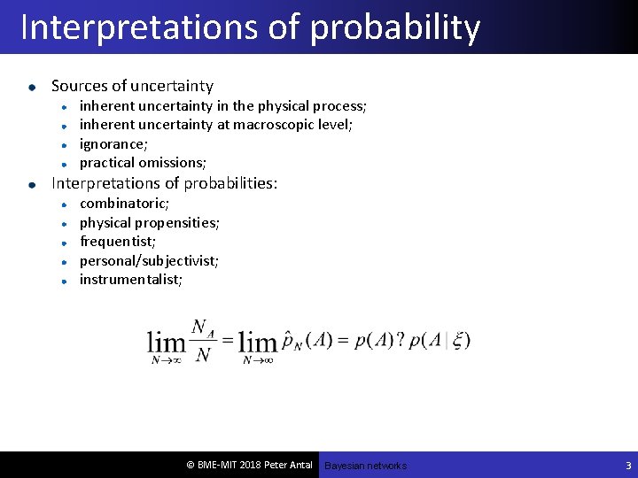
Interpretations of probability Sources of uncertainty inherent uncertainty in the physical process; inherent uncertainty at macroscopic level; ignorance; practical omissions; Interpretations of probabilities: combinatoric; physical propensities; frequentist; personal/subjectivist; instrumentalist; © BME-MIT 2018 Peter Antal Bayesian networks 3

A chronology of uncertain inference [1713] Ars Conjectandi (The Art of Conjecture), Jacob Bernoulli Subjectivist interpretation of probabilities [1718] The Doctrine of Chances, Abraham de Moivre the first textbook on probability theory Forward predictions • „given a specified number of white and black balls in an urn, what is the probability of drawing a black ball? ” • his own death [1764, posthumous] Essay Towards Solving a Problem in the Doctrine of Chances, Thomas Bayes Backward questions: „given that one or more balls has been drawn, what can be said about the number of white and black balls in the urn” [1812], Théorie analytique des probabilités, Pierre-Simon Laplace General Bayes rule. . . [1933]: A. Kolmogorov: Foundations of the Theory of Probability © BME-MIT 2018 Peter Antal

Basic concepts of probability theory Joint distribution Conditional probability Bayes’ rule Chain rule Marginalization General inference Independence • Conditional independence • Contextual independence October 18, 2021 © BME-MIT 2018 Peter Antal Bayesian networks 5

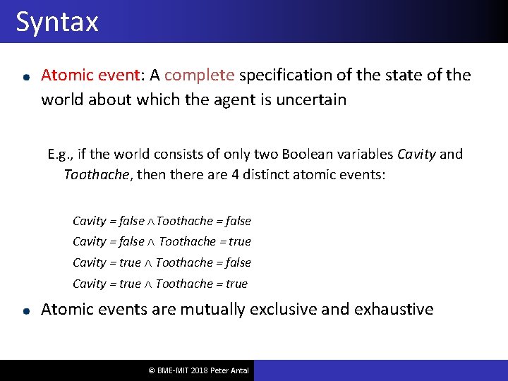
Syntax Atomic event: A complete specification of the state of the world about which the agent is uncertain E. g. , if the world consists of only two Boolean variables Cavity and Toothache, then there are 4 distinct atomic events: Cavity = false Toothache = false Cavity = false Toothache = true Cavity = true Toothache = false Cavity = true Toothache = true Atomic events are mutually exclusive and exhaustive © BME-MIT 2018 Peter Antal

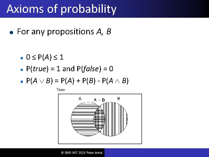
Axioms of probability For any propositions A, B 0 ≤ P(A) ≤ 1 P(true) = 1 and P(false) = 0 P(A B) = P(A) + P(B) - P(A B) © BME-MIT 2018 Peter Antal

Syntax Basic element: random variable Similar to propositional logic: possible worlds defined by assignment of values to random variables. Boolean random variables e. g. , Cavity (do I have a cavity? ) Discrete random variables e. g. , Weather is one of <sunny, rainy, cloudy, snow> Domain values must be exhaustive and mutually exclusive Elementary proposition constructed by assignment of a value to a random variable: e. g. , Weather = sunny, Cavity = false (abbreviated as cavity) Complex propositions formed from elementary propositions and standard logical connectives e. g. , Weather = sunny Cavity = false © BME-MIT 2018 Peter Antal

Joint (probability) distribution Prior or unconditional probabilities of propositions e. g. , P(Cavity = true) = 0. 1 and P(Weather = sunny) = 0. 72 correspond to belief prior to arrival of any (new) evidence Probability distribution gives values for all possible assignments: P(Weather) = <0. 72, 0. 1, 0. 08, 0. 1> (normalized, i. e. , sums to 1) Joint probability distribution for a set of random variables gives the probability of every atomic event on those random variables P(Weather, Cavity) = a 4 × 2 matrix of values: Weather = sunny rainy cloudy snow Cavity = true 0. 144 0. 02 0. 016 0. 02 Cavity = false 0. 576 0. 08 0. 064 0. 08 © BME-MIT 2018 Peter Antal

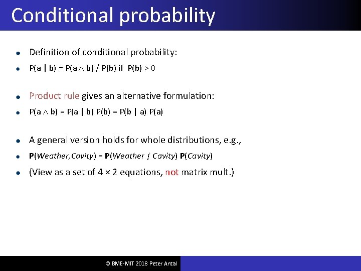
Conditional probability Definition of conditional probability: P(a | b) = P(a b) / P(b) if P(b) > 0 Product rule gives an alternative formulation: P(a b) = P(a | b) P(b) = P(b | a) P(a) A general version holds for whole distributions, e. g. , P(Weather, Cavity) = P(Weather | Cavity) P(Cavity) (View as a set of 4 × 2 equations, not matrix mult. ) © BME-MIT 2018 Peter Antal

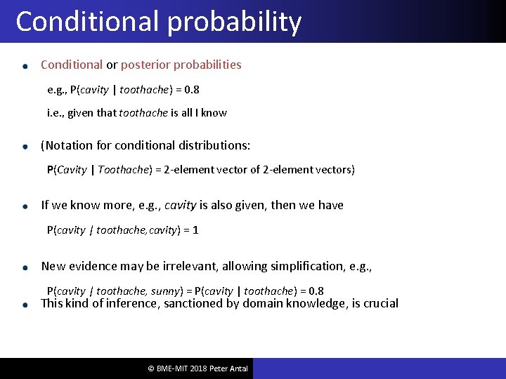
Conditional probability Conditional or posterior probabilities e. g. , P(cavity | toothache) = 0. 8 i. e. , given that toothache is all I know (Notation for conditional distributions: P(Cavity | Toothache) = 2 -element vector of 2 -element vectors) If we know more, e. g. , cavity is also given, then we have P(cavity | toothache, cavity) = 1 New evidence may be irrelevant, allowing simplification, e. g. , P(cavity | toothache, sunny) = P(cavity | toothache) = 0. 8 This kind of inference, sanctioned by domain knowledge, is crucial © BME-MIT 2018 Peter Antal

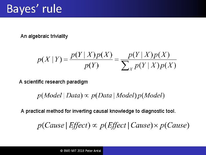
Bayes’ rule An algebraic triviality A scientific research paradigm A practical method for inverting causal knowledge to diagnostic tool. © BME-MIT 2018 Peter Antal

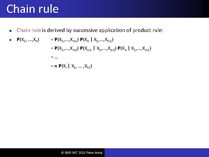
Chain rule is derived by successive application of product rule: P(X 1, …, Xn) = P(X 1, . . . , Xn-1) P(Xn | X 1, . . . , Xn-1) = P(X 1, . . . , Xn-2) P(Xn-1 | X 1, . . . , Xn-2) P(Xn | X 1, . . . , Xn-1) =… = π P(Xi | X 1, … , Xi-1) © BME-MIT 2018 Peter Antal

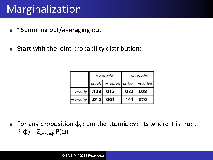
Marginalization ~Summing out/averaging out Start with the joint probability distribution: For any proposition φ, sum the atomic events where it is true: P(φ) = Σω: ω╞φ P(ω) © BME-MIT 2018 Peter Antal

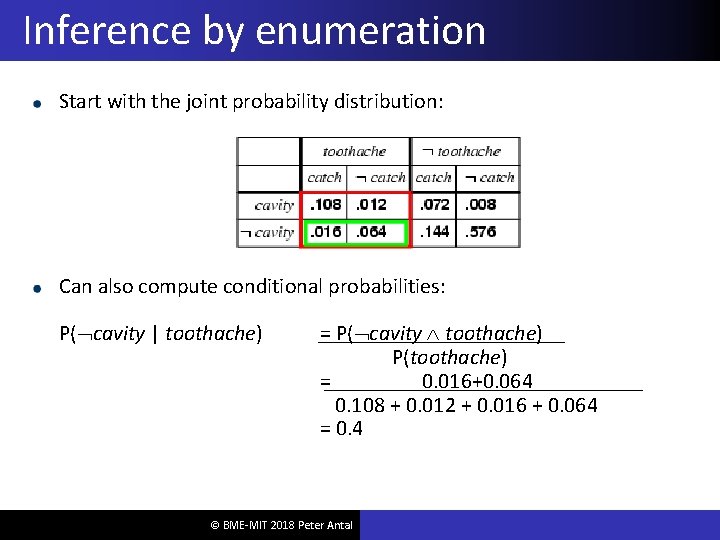
Inference by enumeration Start with the joint probability distribution: Can also compute conditional probabilities: P( cavity | toothache) = P( cavity toothache) P(toothache) = 0. 016+0. 064 0. 108 + 0. 012 + 0. 016 + 0. 064 = 0. 4 © BME-MIT 2018 Peter Antal

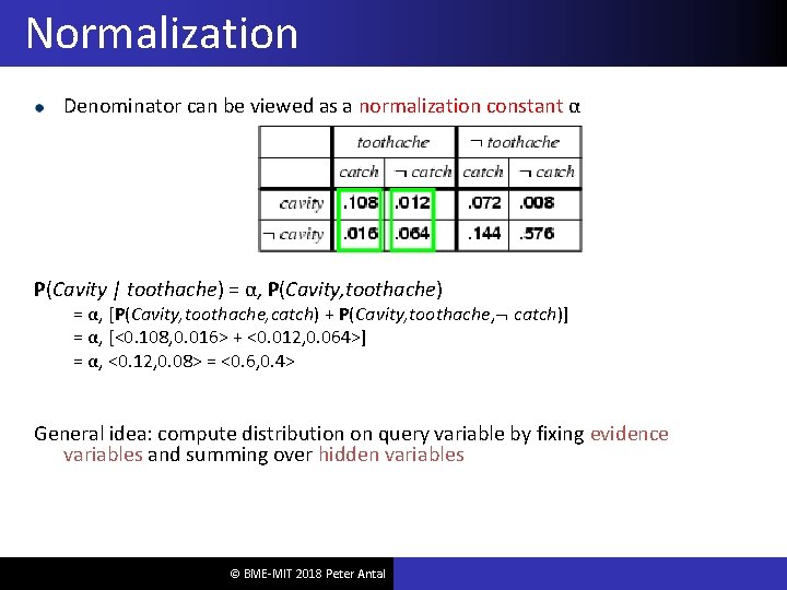
Normalization Denominator can be viewed as a normalization constant α P(Cavity | toothache) = α, P(Cavity, toothache) = α, [P(Cavity, toothache, catch) + P(Cavity, toothache, catch)] = α, [<0. 108, 0. 016> + <0. 012, 0. 064>] = α, <0. 12, 0. 08> = <0. 6, 0. 4> General idea: compute distribution on query variable by fixing evidence variables and summing over hidden variables © BME-MIT 2018 Peter Antal

Inference by enumeration, contd. Any question about observable events in the domain can be answered by the joint distribution. Typically, we are interested in the posterior joint distribution of the query variables Y given specific values e for the evidence variables E Let the hidden variables be H = X - Y – E Then the required summation of joint entries is done by summing out the hidden variables: P(Y | E = e) = αP(Y, E = e) = αΣh. P(Y, E= e, H = h) The terms in the summation are joint entries because Y, E and H together exhaust the set of random variables Obvious problems: 1. 1. 1. Worst-case time complexity O(dn) where d is the largest arity Space complexity O(dn) to store the joint distribution How to find the numbers for O(dn) entries? © BME-MIT 2018 Peter Antal

Independence, Conditional independence IP(X; Y|Z) or (X⫫Y|Z)P denotes that X is independent of Y given Z defined as follows for all x, y and z with P(z)>0: P(x; y|z)=P(x|z) P(y|z) (Almost) alternatively, IP(X; Y|Z) iff P(X|Z, Y)= P(X|Z) for all z, y with P(z, y)>0. Other notations: DP(X; Y|Z) =def= ┐IP(X; Y|Z) Direct dependence: DP(X; Y|V/{X, Y}) © BME-MIT 2018 Peter Antal

Measures of dependence Information theoretic based dependence Entropy: H(X) Conditional entropy: H(X|Y) Kullback-Leibler divergence (KL(p||q)) • Not distance (asymmetric, triangle inequality) • Always positive Mutual information: MI(X; Y), MI(X; Y|Z) • MI(X; Y)=H(X)-H(X|Y) • MI(X; Y)=KL(p(X, Y)||p(X)p(Y)) October 18, 2021 © BME-MIT 2018 Peter Antal A. I. 19

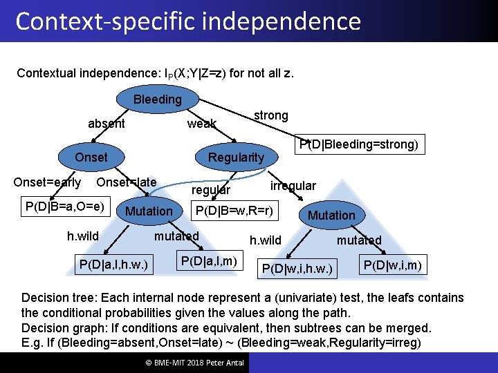
Context-specific independence Contextual independence: IP(X; Y|Z=z) for not all z. Bleeding absent weak Onset=early P(D|Bleeding=strong) Regularity Onset=late P(D|B=a, O=e) strong Mutation h. wild regular P(D|B=w, R=r) mutated P(D|a, l, h. w. ) irregular P(D|a, l, m) Mutation h. wild P(D|w, i, h. w. ) mutated P(D|w, i, m) Decision tree: Each internal node represent a (univariate) test, the leafs contains the conditional probabilities given the values along the path. Decision graph: If conditions are equivalent, then subtrees can be merged. E. g. If (Bleeding=absent, Onset=late) ~ (Bleeding=weak, Regularity=irreg) © BME-MIT 2018 Peter Antal

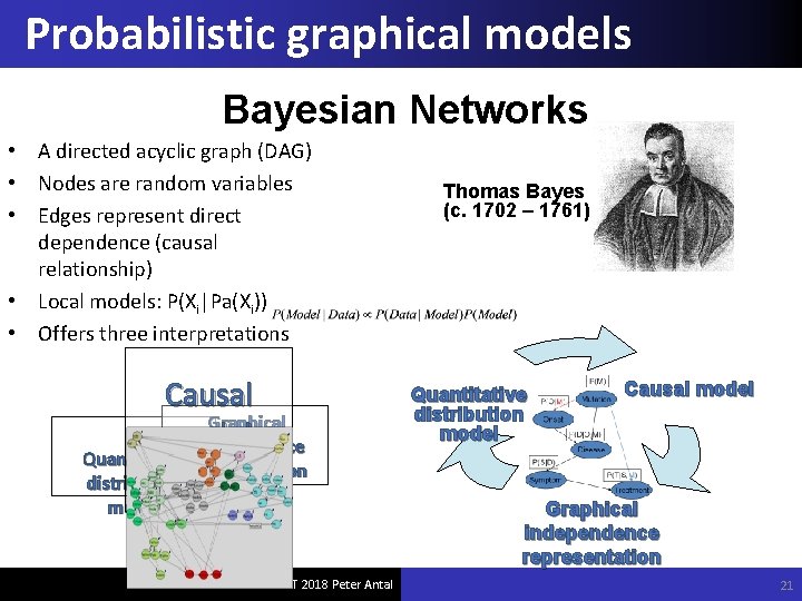
Probabilistic graphical models Bayesian Networks • A directed acyclic graph (DAG) • Nodes are random variables • Edges represent direct dependence (causal relationship) • Local models: P(Xi|Pa(Xi)) • Offers three interpretations Causal Graphical model independence Quantitative representation distribution model © BME-MIT 2018 Peter Antal Thomas Bayes (c. 1702 – 1761) Quantitative distribution model Causal model Graphical independence representation 21

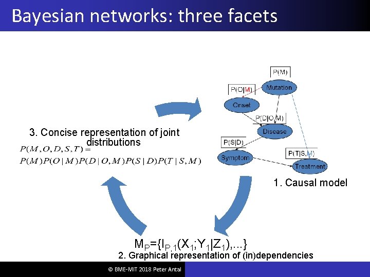
Bayesian networks: three facets 3. Concise representation of joint distributions 1. Causal model MP={IP, 1(X 1; Y 1|Z 1), . . . } 2. Graphical representation of (in)dependencies © BME-MIT 2018 Peter Antal

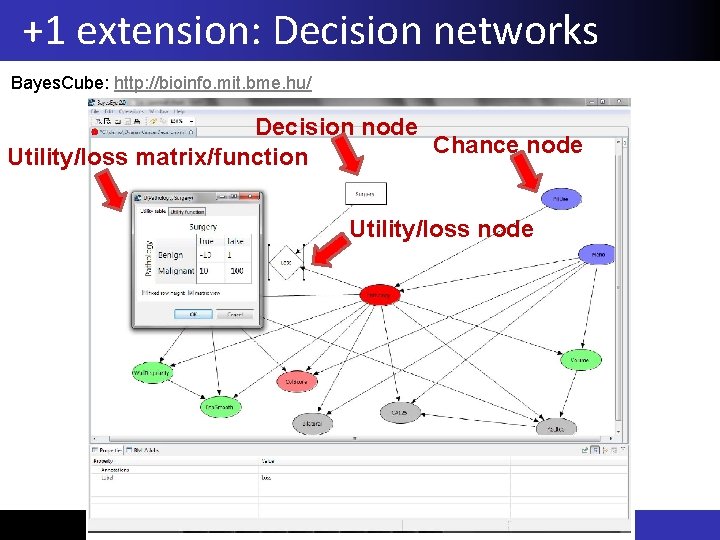
+1 extension: Decision networks Bayes. Cube: http: //bioinfo. mit. bme. hu/ Decision node Chance node Utility/loss matrix/function Utility/loss node © BME-MIT 2018 Peter Antal

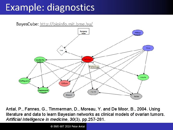
Example: diagnostics Bayes. Cube: http: //bioinfo. mit. bme. hu/ Antal, P. , Fannes, G. , Timmerman, D. , Moreau, Y. and De Moor, B. , 2004. Using literature and data to learn Bayesian networks as clinical models of ovarian tumors. Artificial Intelligence in medicine, 30(3), pp. 257 -281. © BME-MIT 2018 Peter Antal

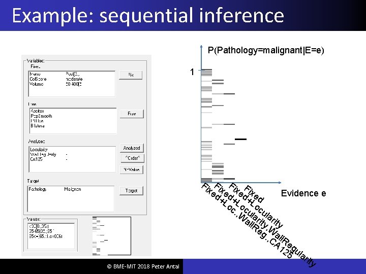
Example: sequential inference P(Pathology=malignant|E=e) 1 © BME-MIT 2018 Peter Antal Fi Fi Fi F xe xe xe ix Evidence e d+ d+ d+ ed Lo Lo Lo c. , cu cu W lar all ity Re , W g. al , C l. R A 1 eg 25 ula rit y

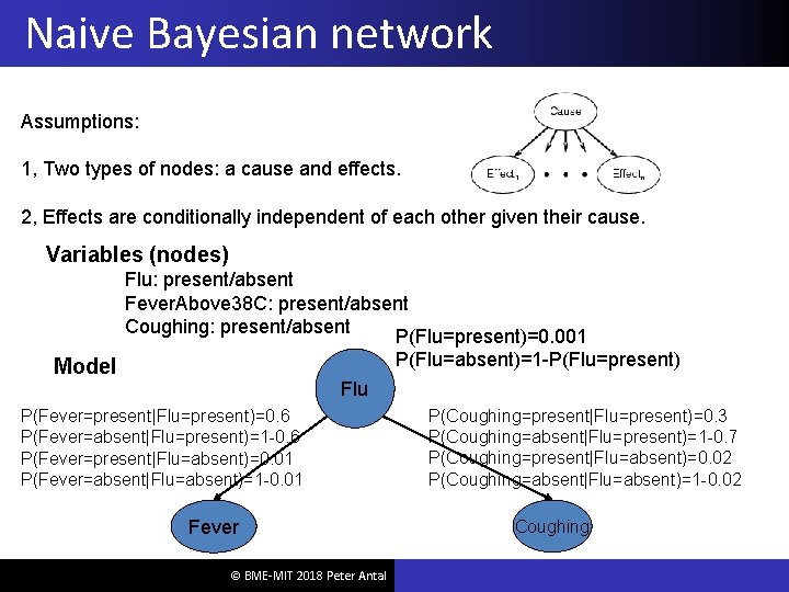
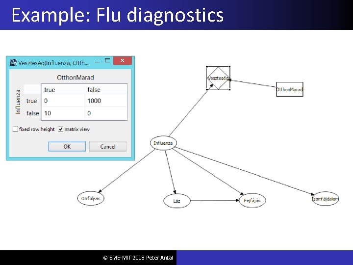
Naive Bayesian network Assumptions: 1, Two types of nodes: a cause and effects. 2, Effects are conditionally independent of each other given their cause. Variables (nodes) Flu: present/absent Fever. Above 38 C: present/absent Coughing: present/absent P(Flu=present)=0. 001 P(Flu=absent)=1 -P(Flu=present) Model Flu P(Fever=present|Flu=present)=0. 6 P(Fever=absent|Flu=present)=1 -0. 6 P(Fever=present|Flu=absent)=0. 01 P(Fever=absent|Flu=absent)=1 -0. 01 Fever © BME-MIT 2018 Peter Antal P(Coughing=present|Flu=present)=0. 3 P(Coughing=absent|Flu=present)=1 -0. 7 P(Coughing=present|Flu=absent)=0. 02 P(Coughing=absent|Flu=absent)=1 -0. 02 Coughing

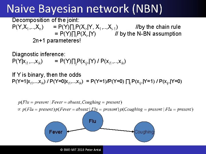
Naive Bayesian network (NBN) Decomposition of the joint: P(Y, X 1, . . , Xn) = P(Y)∏i. P(Xi, |Y, X 1, . . , Xi-1) //by the chain rule = P(Y)∏i. P(Xi, |Y) // by the N-BN assumption 2 n+1 parameteres! Diagnostic inference: P(Y|xi 1, . . , xik) = P(Y)∏j. P(xij, |Y) / P(xi 1, . . , xik) If Y is binary, then the odds P(Y=1|xi 1, . . , xik) / P(Y=0|xi 1, . . , xik) = P(Y=1)/P(Y=0) ∏j P(xij, |Y=1) / P(xij, |Y=0) Flu Fever © BME-MIT 2018 Peter Antal Coughing

Example: SPAM filter NBN SPAM filter SPAM: yes/no [suspicious. . ] Attributes • Sender, subject, link, attachment, . . © BME-MIT 2018 Peter Antal

Example: Flu diagnostics © BME-MIT 2018 Peter Antal

Markov processes (Markov chains) © BME-MIT 2018 Peter Antal Bayesian networks 30

Hidden Markov Models (HMMs) © BME-MIT 2018 Peter Antal Bayesian networks 31

HMMs: definition © BME-MIT 2018 Peter Antal Bayesian networks 32

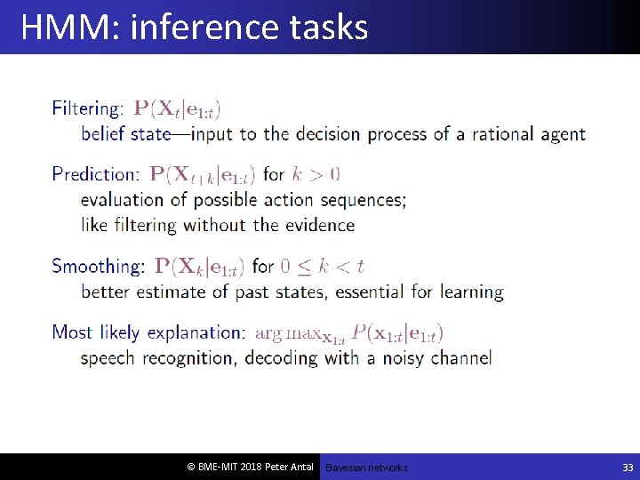
HMM: inference tasks © BME-MIT 2018 Peter Antal Bayesian networks 33

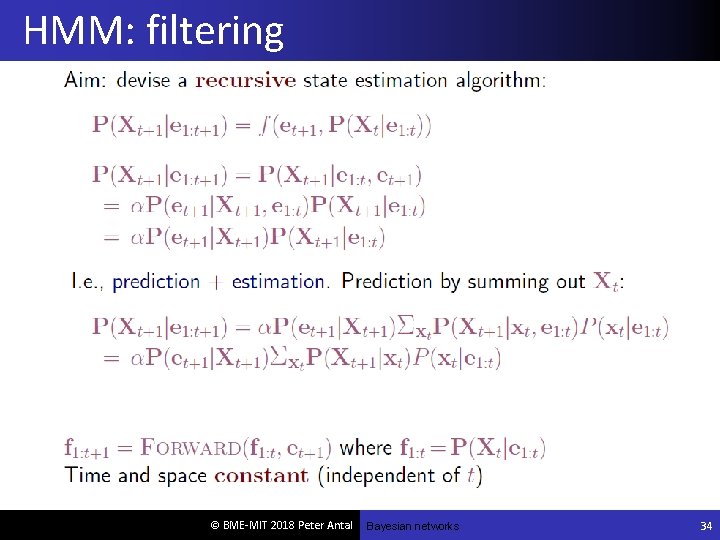
HMM: filtering © BME-MIT 2018 Peter Antal Bayesian networks 34

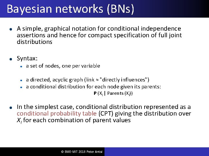
Bayesian networks (BNs) A simple, graphical notation for conditional independence assertions and hence for compact specification of full joint distributions Syntax: a set of nodes, one per variable a directed, acyclic graph (link ≈ "directly influences") a conditional distribution for each node given its parents: P (Xi | Parents (Xi)) In the simplest case, conditional distribution represented as a conditional probability table (CPT) giving the distribution over Xi for each combination of parent values © BME-MIT 2018 Peter Antal

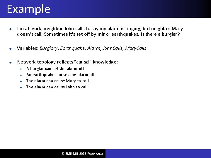
Example I'm at work, neighbor John calls to say my alarm is ringing, but neighbor Mary doesn't call. Sometimes it's set off by minor earthquakes. Is there a burglar? Variables: Burglary, Earthquake, Alarm, John. Calls, Mary. Calls Network topology reflects "causal" knowledge: A burglar can set the alarm off An earthquake can set the alarm off The alarm can cause Mary to call The alarm can cause John to call © BME-MIT 2018 Peter Antal

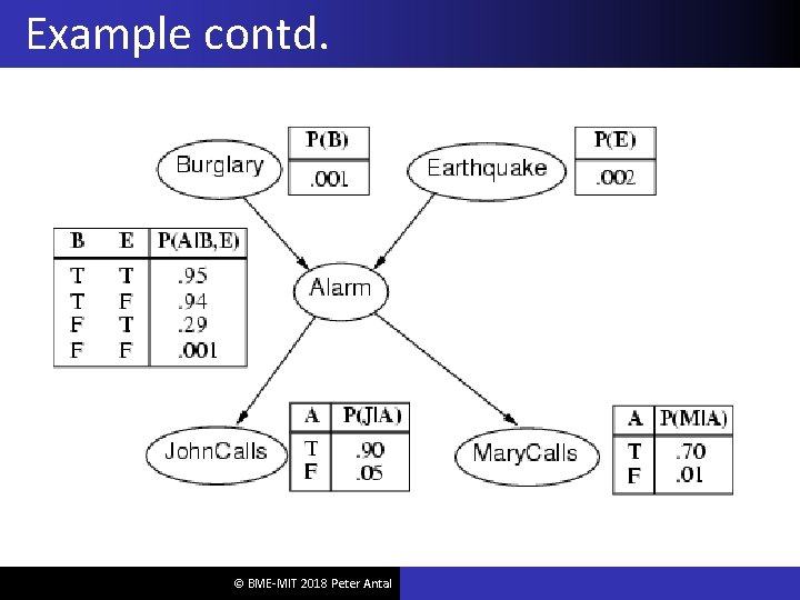
Example contd. © BME-MIT 2018 Peter Antal

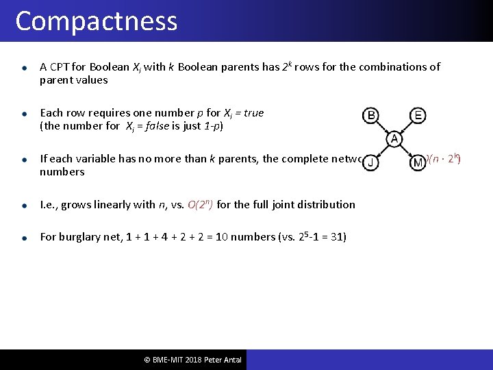
Compactness A CPT for Boolean Xi with k Boolean parents has 2 k rows for the combinations of parent values Each row requires one number p for Xi = true (the number for Xi = false is just 1 -p) If each variable has no more than k parents, the complete network requires O(n · 2 k) numbers I. e. , grows linearly with n, vs. O(2 n) for the full joint distribution For burglary net, 1 + 4 + 2 = 10 numbers (vs. 25 -1 = 31) © BME-MIT 2018 Peter Antal

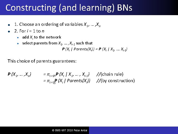
Constructing (and learning) BNs 1. Choose an ordering of variables X 1, … , Xn 2. For i = 1 to n add Xi to the network select parents from X 1, … , Xi-1 such that P (Xi | Parents(Xi)) = P (Xi | X 1, . . . Xi-1) This choice of parents guarantees: P (X 1, … , Xn) = πi =1 n P (Xi | X 1, … , Xi-1) = πi =1 n. P (Xi | Parents(Xi)) © BME-MIT 2018 Peter Antal //(chain rule) //(by construction)

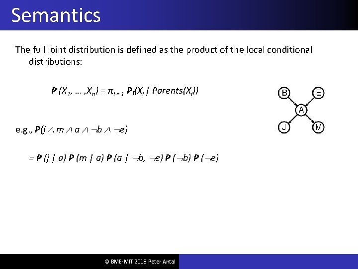
Semantics The full joint distribution is defined as the product of the local conditional distributions: P (X 1, … , Xn) = πi = 1 P n(Xi | Parents(Xi)) e. g. , P(j m a b e) = P (j | a) P (m | a) P (a | b, e) P ( b) P ( e) © BME-MIT 2018 Peter Antal

Local models in BNs: Noisy-OR © BME-MIT 2018 Peter Antal

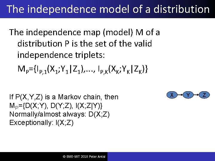
The independence model of a distribution The independence map (model) M of a distribution P is the set of the valid independence triplets: MP={IP, 1(X 1; Y 1|Z 1), . . . , IP, K(XK; YK|ZK)} If P(X, Y, Z) is a Markov chain, then MP={D(X; Y), D(Y; Z), I(X; Z|Y)} Normally/almost always: D(X; Z) Exceptionally: I(X; Z) © BME-MIT 2018 Peter Antal X Y Z

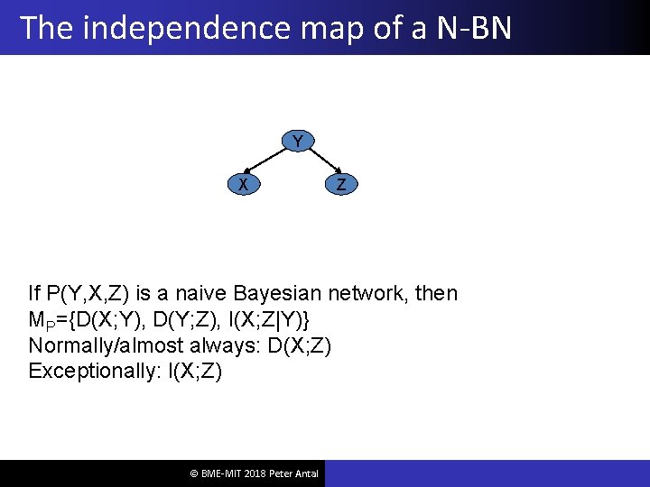
The independence map of a N-BN Y X Z If P(Y, X, Z) is a naive Bayesian network, then MP={D(X; Y), D(Y; Z), I(X; Z|Y)} Normally/almost always: D(X; Z) Exceptionally: I(X; Z) © BME-MIT 2018 Peter Antal

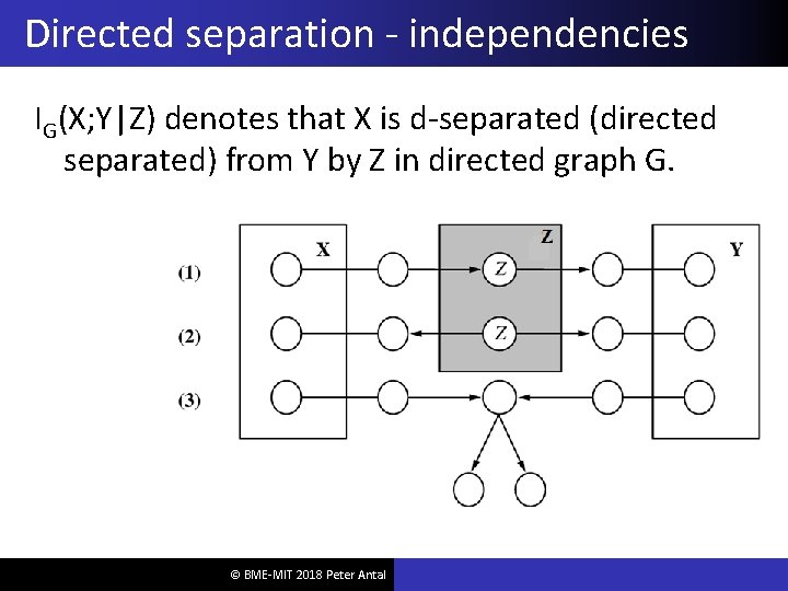
Directed separation - independencies IG(X; Y|Z) denotes that X is d-separated (directed separated) from Y by Z in directed graph G. © BME-MIT 2018 Peter Antal

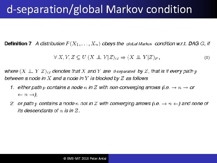
d-separation/global Markov condition © BME-MIT 2018 Peter Antal

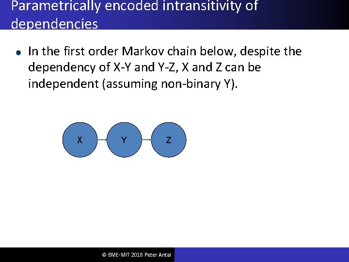
Parametrically encoded intransitivity of dependencies In the first order Markov chain below, despite the dependency of X-Y and Y-Z, X and Z can be independent (assuming non-binary Y). X Y Z © BME-MIT 2018 Peter Antal

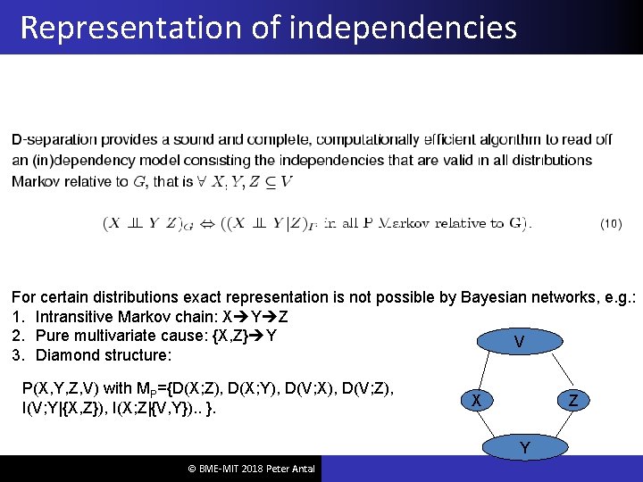
Representation of independencies For certain distributions exact representation is not possible by Bayesian networks, e. g. : 1. Intransitive Markov chain: X Y Z 2. Pure multivariate cause: {X, Z} Y V 3. Diamond structure: P(X, Y, Z, V) with MP={D(X; Z), D(X; Y), D(V; X), D(V; Z), I(V; Y|{X, Z}), I(X; Z|{V, Y}). . }. X Z Y © BME-MIT 2018 Peter Antal

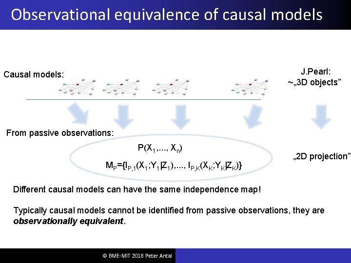
Observational equivalence of causal models J. Pearl: ~„ 3 D objects” Causal models: From passive observations: P(X 1, . . . , Xn) MP={IP, 1(X 1; Y 1|Z 1), . . . , IP, K(XK; YK|ZK)} „ 2 D projection” Different causal models can have the same independence map! Typically causal models cannot be identified from passive observations, they are observationally equivalent. © BME-MIT 2018 Peter Antal

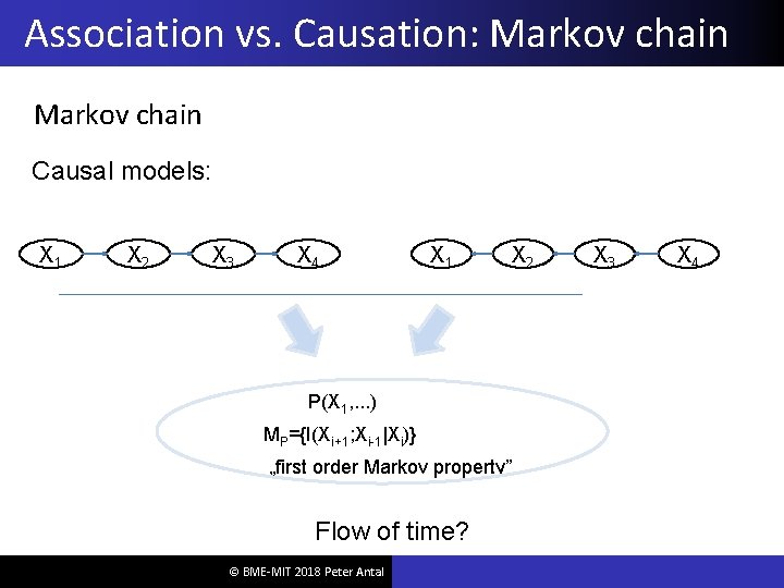
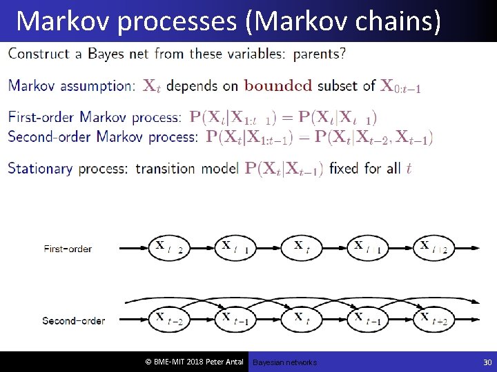
Association vs. Causation: Markov chain Causal models: X 1 X 2 X 3 X 4 X 1 P(X 1, . . . ) MP={I(Xi+1; Xi-1|Xi)} „first order Markov property” Flow of time? © BME-MIT 2018 Peter Antal X 2 X 3 X 4

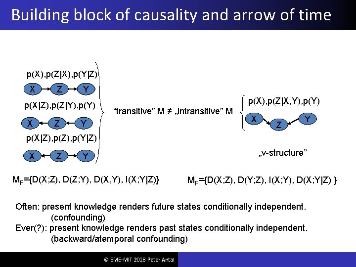
Building block of causality and arrow of time p(X), p(Z|X), p(Y|Z) X Z Y p(X|Z), p(Z|Y), p(Y) X Z p(X), p(Z|X, Y), p(Y) “transitive” M ≠ „intransitive” M Y X Z Y p(X|Z), p(Y|Z) X Z „v-structure” Y MP={D(X; Z), D(Z; Y), D(X, Y), I(X; Y|Z)} MP={D(X; Z), D(Y; Z), I(X; Y), D(X; Y|Z) } Often: present knowledge renders future states conditionally independent. (confounding) Ever(? ): present knowledge renders past states conditionally independent. (backward/atemporal confounding) © BME-MIT 2018 Peter Antal

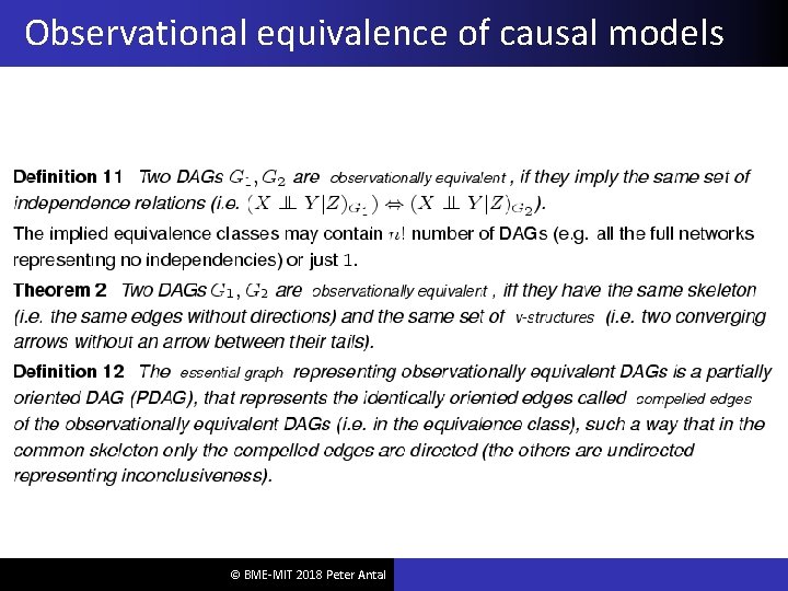
Observational equivalence of causal models © BME-MIT 2018 Peter Antal

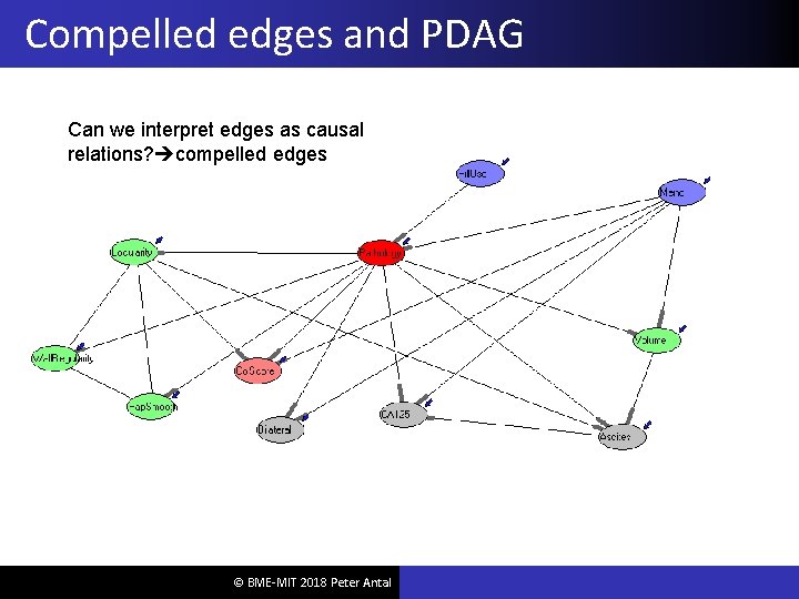
Compelled edges and PDAG Can we interpret edges as causal relations? compelled edges © BME-MIT 2018 Peter Antal

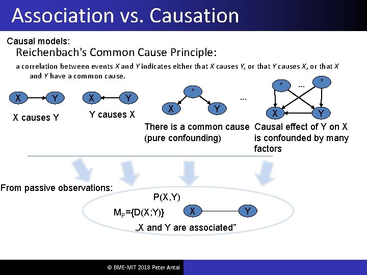
Association vs. Causation Causal models: Reichenbach's Common Cause Principle: a correlation between events X and Y indicates either that X causes Y, or that Y causes X, or that X and Y have a common cause. X Y X causes Y X * Y Y causes X From passive observations: * X . . . * . . . Y X Y There is a common cause Causal effect of Y on X is confounded by many (pure confounding) factors P(X, Y) MP={D(X; Y)} X „X and Y are associated” © BME-MIT 2018 Peter Antal Y

Inference in BNs 10/18/2021 Bayesian networks 59/x

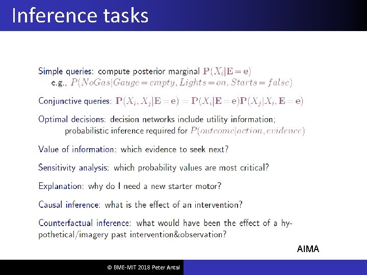
Inference tasks AIMA © BME-MIT 2018 Peter Antal

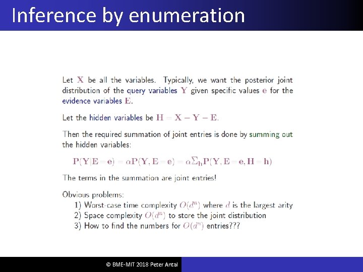
Inference by enumeration © BME-MIT 2018 Peter Antal

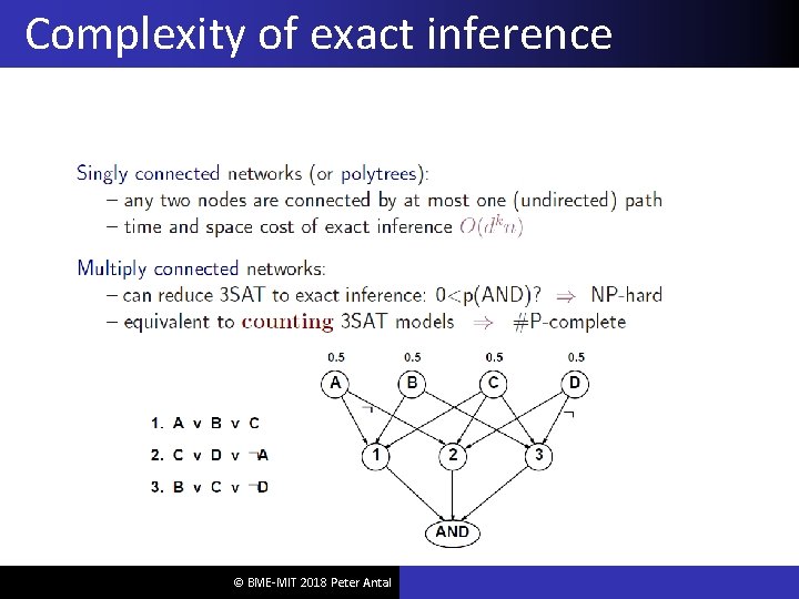
Complexity of exact inference © BME-MIT 2018 Peter Antal

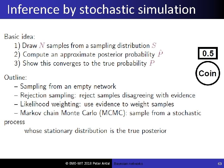
Inference by stochastic simulation © BME-MIT 2018 Peter Antal Bayesian networks 63

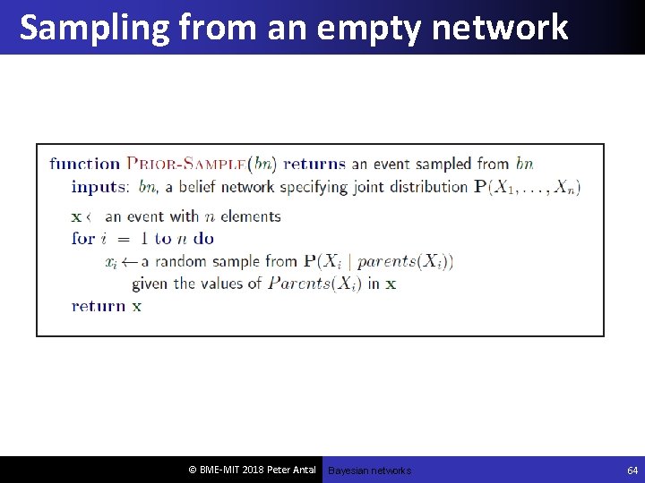
Sampling from an empty network © BME-MIT 2018 Peter Antal Bayesian networks 64

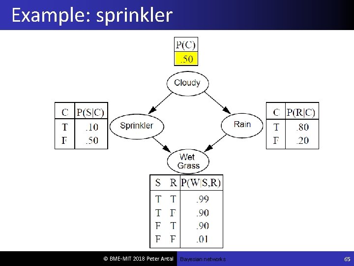
Example: sprinkler © BME-MIT 2018 Peter Antal Bayesian networks 65

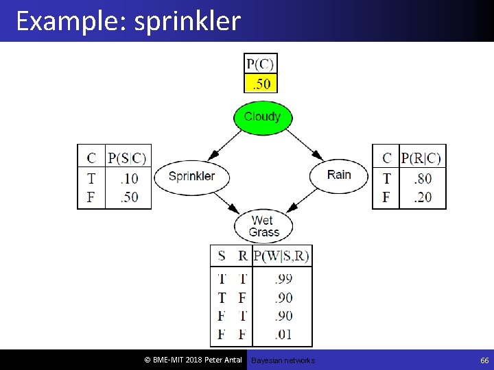
Example: sprinkler © BME-MIT 2018 Peter Antal Bayesian networks 66

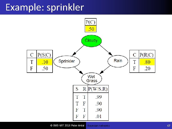
Example: sprinkler © BME-MIT 2018 Peter Antal Bayesian networks 67

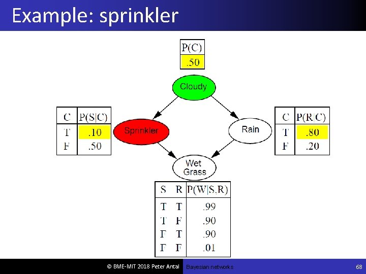
Example: sprinkler © BME-MIT 2018 Peter Antal Bayesian networks 68

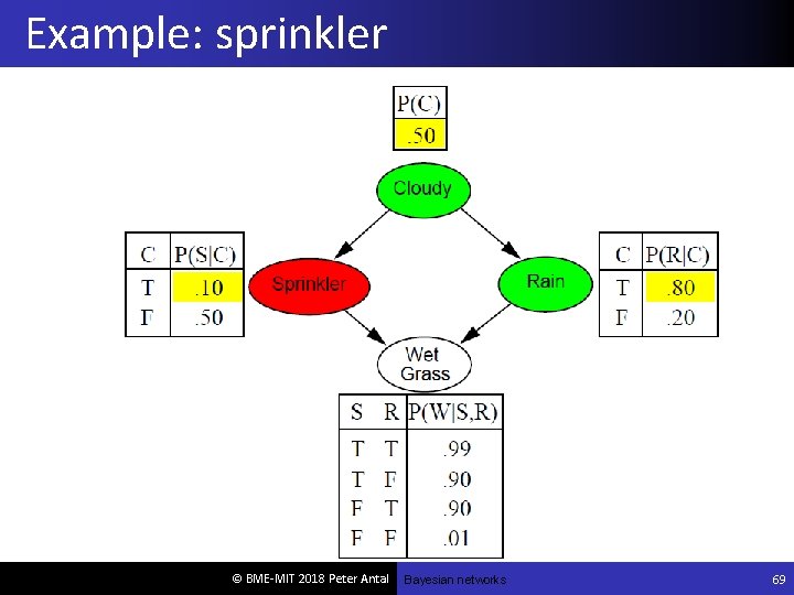
Example: sprinkler © BME-MIT 2018 Peter Antal Bayesian networks 69

Example: sprinkler © BME-MIT 2018 Peter Antal Bayesian networks 70

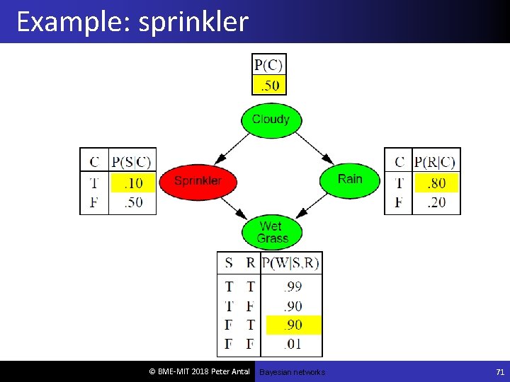
Example: sprinkler © BME-MIT 2018 Peter Antal Bayesian networks 71

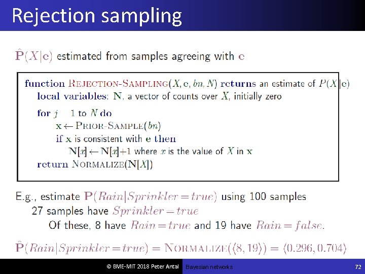
Rejection sampling © BME-MIT 2018 Peter Antal Bayesian networks 72

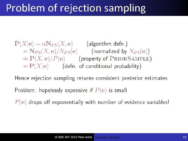
Problem of rejection sampling © BME-MIT 2018 Peter Antal Bayesian networks 73

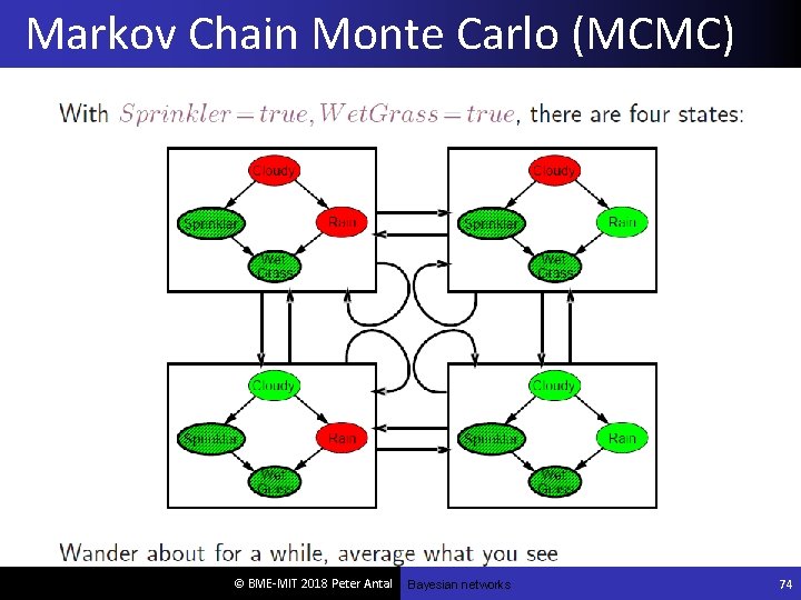
Markov Chain Monte Carlo (MCMC) © BME-MIT 2018 Peter Antal Bayesian networks 74

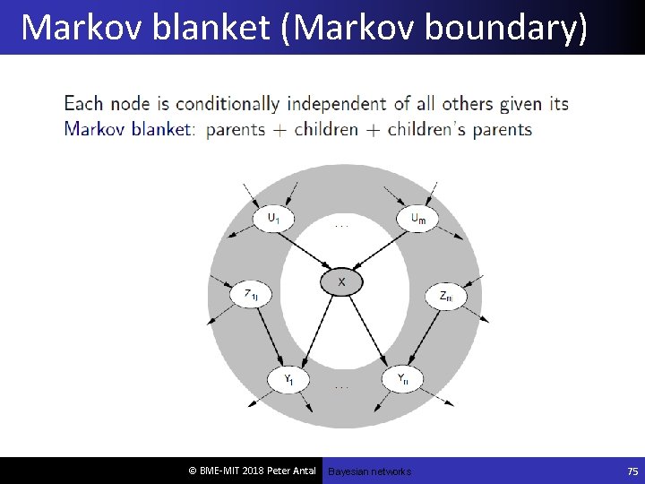
Markov blanket (Markov boundary) © BME-MIT 2018 Peter Antal Bayesian networks 75

Approximate inference using MCMC © BME-MIT 2018 Peter Antal Bayesian networks 76

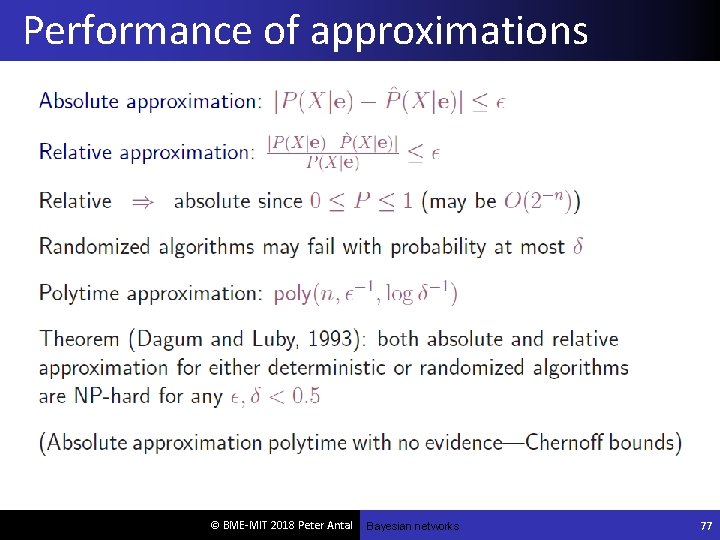
Performance of approximations © BME-MIT 2018 Peter Antal Bayesian networks 77

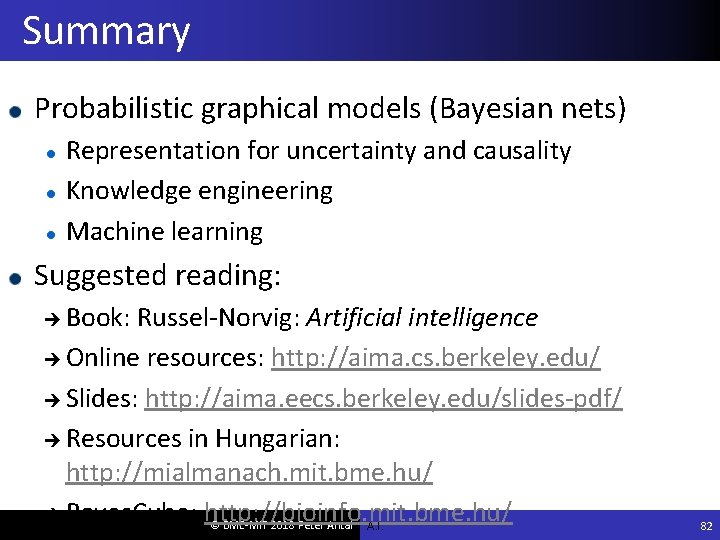
Summary Probabilistic graphical models (Bayesian nets) Representation for uncertainty and causality Knowledge engineering Machine learning Suggested reading: Book: Russel-Norvig: Artificial intelligence Online resources: http: //aima. cs. berkeley. edu/ Slides: http: //aima. eecs. berkeley. edu/slides-pdf/ Resources in Hungarian: http: //mialmanach. mit. bme. hu/ Bayes. Cube: http: //bioinfo. mit. bme. hu/ © BME-MIT 2018 Peter Antal A. I. 82