Artificial Intelligence A Modern Approach Problem Solving II

Informed Search Strategies

Best-first search Best first search is an instance of the general TREE-SEARCH or GRAPH-SEARCH algorithm in which a node is selected for expansion based on an evaluation function, f(n). A Key component of these algorithms is a heuristic function, h (n): h (n) = estimated cost of the cheapest path from node n to a goal node. • The two types of evaluation functions are: – Expand the node closest to the goal state using estimated cost as the evaluation is called Greedy best-first search. – Expand the node on the least cost solution path using estimated cost and actual cost as the evaluation function is called A* search.

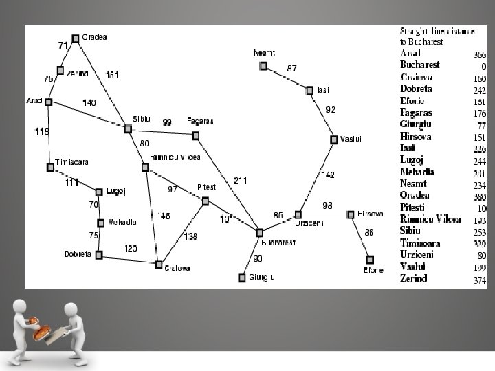
Greedy best-first search tries to expand the node that is closest to the goal, on the grounds that this is likely to lead to a solution quickly. Thus, it evaluates nodes by using just the heuristic function: f (n) = h (n). A* search: Minimizing the total estimated solution cost Expand the node on the least cost solution path using estimated cost and actual cost as the evaluation function is called A* search. f (n) = g (n) + h (n). since g (n) gives the path cost from the start node to node n, and h (n) is the estimated cost of the cheapest path from n to the goal,

Greedy Best-First Search

A* Search A* S E A R C H

Memory Bounded Heuristic Search • The memory requirements of A* is reduced by combining the heuristic function with iterative deepening resulting an IDA* algorithm. • The two recent memory bounded algorithms are: 1. Recursive best-first search(RBFS) 2. Memory bounded A* search (MA*)

Recursive best-first search(RBFS)

Recursive best-first search(RBFS) • RBFS is simple recursive algorithm uses only linear space. function RECURSIVE-BEST-FIRST-SEARCH(problem) returns a solution, or failure RBFS (problem, MAKE-NODE (INITIAL-STATE [problem]), ∞) function RBFS(problem, node, f_limit) returns a solution, or failure and a new f-cost limit if GOAL-TEST[problem](state) then return node successors ← EXPAND (node, problem) if successors is empty then return failure, ∞ for each s in successors do f[s] ← max(g(s) + h(s). f[node]) repeat best ← the lowest f-value node in successors if f[best] > f_limit then return failure, f[best] alternative ← the second-lowest f-value among successors result, f[best] ← RBFS(problem, best, min(f_limit, alternative)) if result ≠ failure then return result

• Search techniques which use all available memory are: – – MA* (Memory-bounded A*) SMA* (Simplified MA*) • SMA* (Simplified MA*) It can make use of all available memory to carry out the search. Properties: i) It will utilize whatever memory is made available to it. ii) It avoids repeated states as far as its memory allows. Advantage: SMA* uses only the available memory. Disadvantage: If enough memory is not available it leads to suboptimal solution. Space and Time complexity: depends on the available number of nodes

Heuristic Functions Task: Find the shortest solution using heuristic function that never over estimates the number of steps to the goal. Solution: To perform the given task two candidates are required, which are named as h 1 and h 2 • h 1 = the number of misplaced tiles. From figure, all of the eight tiles are out of position, so the start state would have h 1 = 8. h 1 is an admissible heuristic, because it is clear that any tile that is out of place must be moved at least once. • h 2 = the sum of the distances of the tiles from their goal positions. The sum of the distances of the tiles from their goal positions is called as city block distance or Manhattan distance of: h 2 = 3 + 1 + 2 + 2 + 3 + 2 = 18

Heuristic Functions • Branching Factor • Relaxed Problem • Absolver • Pattern Databases • Learning Heuristics from experience

Local Search Algorithms and Optimization Problems

Local Search Algorithms and Optimization Problems • Local search algorithms operate using a single current state and generally move only to neighbors of that state. • Two Key Advantages: – They use very little memory – usually a constant amount – They can often find reasonable solutions in large or infinite (continuous) state spaces for which systematic algorithms are unsuitable.

Local Search Algorithms • Hill climbing search • Simulated annealing • • Local beam search • Genetic algorithm(GA)

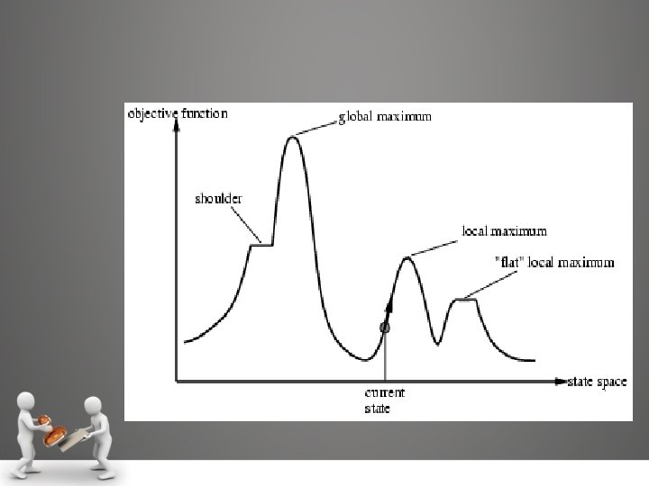
Hill climbing search

Hill Climbing- 8 Queens Problem

Simulated Annealing Search • An algorithm which combines hill climbing with random walk to yield both efficiency and completeness. This algorithm was developed using annealing process the process of gradually cooling a liquid until it freezes.

Simulated Annealing Search Applications: • VLSI layout • Airline scheduling

Local Beam Search • The Local beam search algorithm keeps track of k states rather than just one. It begins with k randomly generated states. At each step, all the successors of all k states are generated. If any one is a goal, the algorithm halts. Otherwise, it selects the k best successors from the complete list and repeats. In a local beam search, useful information is passed among the k parallel search threads. • This search will suffer from lack of diversity among k states. Therefore a variant named as stochastic beam search selects k successors at random, with the probability of choosing a given successor being an increasing function of its value.

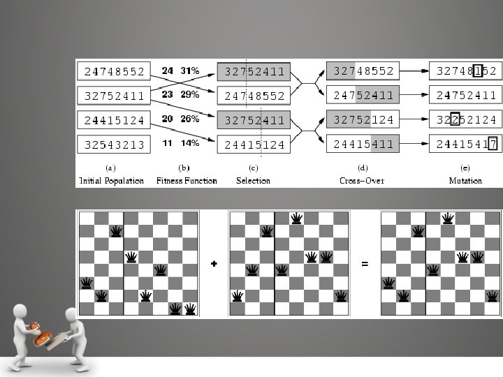
Genetic Algorithm • A GA is a variant of stochastic beam search in which successor states are generated by combining two parent states, rather than by modifying a single state. Figure describes a GA algorithm.

Local Search in Continuous Space

Online Search Agents

Online Search Agents and Unknown Environments • Offline search: They compute a complete solution before setting foot in the real world, and then execute the solution without recourse to their percepts. • Online search: Agents operate by interleaving computation and action: first it takes an action, and then it observes the environment and computes the next action. • Online search is a good idea in dynamic or semi dynamic domains and stochastic domains. • Online search is a necessary idea for an exploration problem, where the states and actions are unknown to the agent.

Online Search Agents and Unknown Environments • Online Search Problems • Online Search Agents • Online Local Search • Learning in Online Search

Online Search Problems • An online search problem can be solved only by an agent executing actions, rather than by a purely computational process. We will assume that the agent knows just the following: – ACTIONS(s), which returns a list of actions allowed in state in s; – The step-cost function c(s, a, s‘) known to the agent when it reaches s‘ – GOAL-TEST(s). • Here the agent cannot access the successors of a state, except by trying all possible actions in that state. This drawback of an agent can be avoided by: • – Visited states are known to the agent. – Actions are deterministic. – Possible to find Manhattan distance heuristic. E. g. A simple maze problem

Online Search Agents • An online algorithm, expand only a node that it physically occupies. After each action, an online agent receives a percept to know the state it has reached and it can augment its map of the environment, to decide where to go next. • An online depth-first search agent is shown in figure. • function ONLINE-DFS_AGENT(s’) returns an action • inputs: s’, a percept that identifies the current state • static: result, a table, indexed by action and state, initially empty • unexplored, a table that lists, for each visited state, the actions not yet tried • unbacktracked, a table that lists, for each visited state, the backtracks not yet tried • s, a, the previous state and action, initially null • if GOAL-TEST(s’) then return stop • if s’ is a new state then unexplored[s’] ← ACTION(s’) • if s is not null then do • result[a, s] ← s’

Online Local Search • Hill climbing search technique can be used to perform online local search because it keeps just one current state in memory. To avoid the drawback of local maxima, random walk is chosen to explore the environment instead of random restart method. The concept of hill climbing with memory stores a ―current best estimate‖ H(s) of the cost to reach the goal from each state that has been visited is implemented as Learning Real-Time A* (LRTA*) algorithm.

Constraint satisfaction problems (CSP)

Constraint satisfaction problems (CSP) • Constraint satisfaction problems (CSP) is defined by a set of variables, X 1, X 2, …Xn, and a set of constraints, C 1, C 2, …Cm. Each variable Xi has a nonempty domain Di of all possible values. A complete assignment is one in which every variable is mentioned, and a solution to a CSP is a complete assignment that satisfies all the constraints. Some CSPs also require a solution that maximizes an objective function. • Some examples for CSP‘s are: – The n-queens problem – A crossword problem – A map coloring problem

Backtracking Search for CSP’s • Backtracking search, a form of depth first search that chooses values for one variable at a time and backtracks when a variable has no legal values left to assign.