Arrays Records and Pointers Arrays Records and Pointers

Arrays, Records and Pointers

Arrays, Records and Pointers • Data structures are classified as either linear or nonlinear. • Normally arrays and linked lists fall into linear data structures. • Trees and graphs are treated as nonlinear structures.

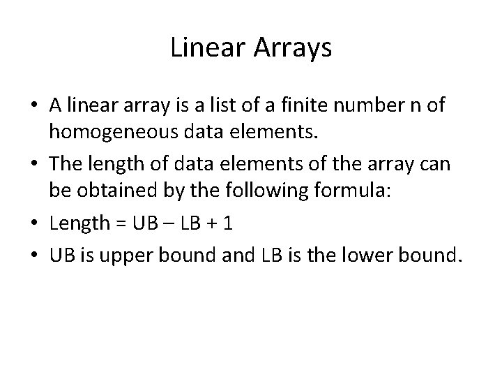
Linear Arrays • A linear array is a list of a finite number n of homogeneous data elements. • The length of data elements of the array can be obtained by the following formula: • Length = UB – LB + 1 • UB is upper bound and LB is the lower bound.

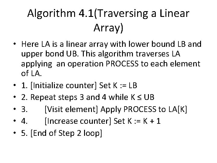
Algorithm 4. 1(Traversing a Linear Array) • Here LA is a linear array with lower bound LB and upper bond UB. This algorithm traverses LA applying an operation PROCESS to each element of LA. • 1. [Initialize counter] Set K : = LB • 2. Repeat steps 3 and 4 while K ≤ UB • 3. [Visit element] Apply PROCESS to LA[K] • 4. [Increase counter] Set K : = K + 1 • 5. [End of Step 2 loop]

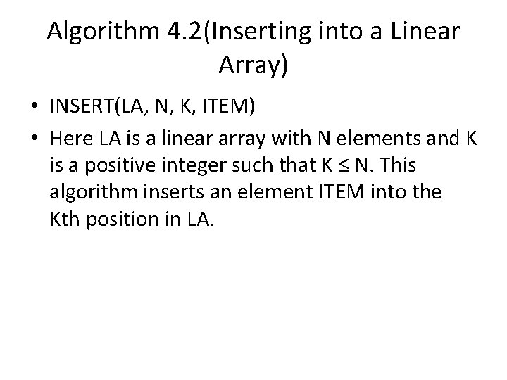
Algorithm 4. 2(Inserting into a Linear Array) • INSERT(LA, N, K, ITEM) • Here LA is a linear array with N elements and K is a positive integer such that K ≤ N. This algorithm inserts an element ITEM into the Kth position in LA.

Algorithm 4. 2(Inserting into a Linear Array) • • • 1. [Initialize counter] Set J : = N 2. Repeat steps 3 and 4 while J ≥ K [Move Jth element downward] 3. Set LA[J+1] : = LA[J] 4. [Decrease counter] Set J : = J – 1 [End of Step 2 loop] 5. [Insert element] Set LA[K] : = ITEM 6. [Reset N] Set N : = N + 1 7. Exit

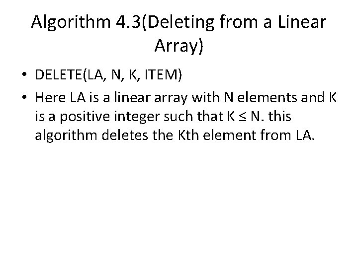
Algorithm 4. 3(Deleting from a Linear Array) • DELETE(LA, N, K, ITEM) • Here LA is a linear array with N elements and K is a positive integer such that K ≤ N. this algorithm deletes the Kth element from LA.

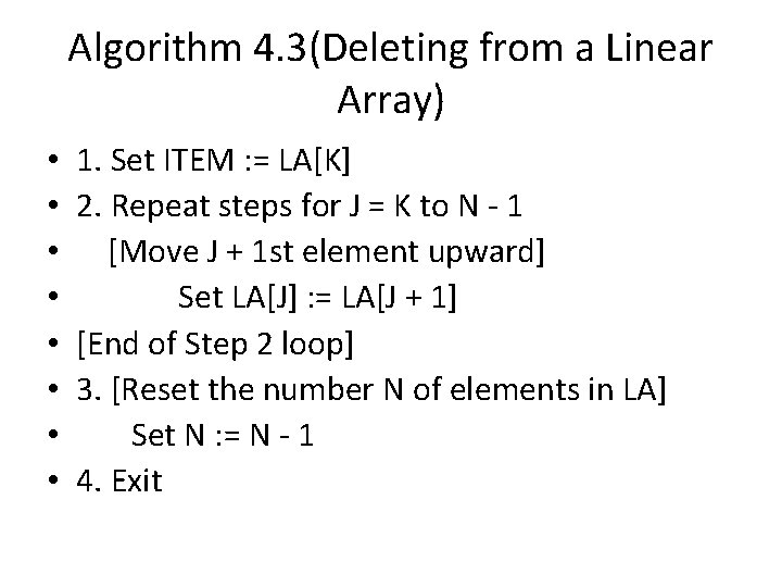
Algorithm 4. 3(Deleting from a Linear Array) • • 1. Set ITEM : = LA[K] 2. Repeat steps for J = K to N - 1 [Move J + 1 st element upward] Set LA[J] : = LA[J + 1] [End of Step 2 loop] 3. [Reset the number N of elements in LA] Set N : = N - 1 4. Exit

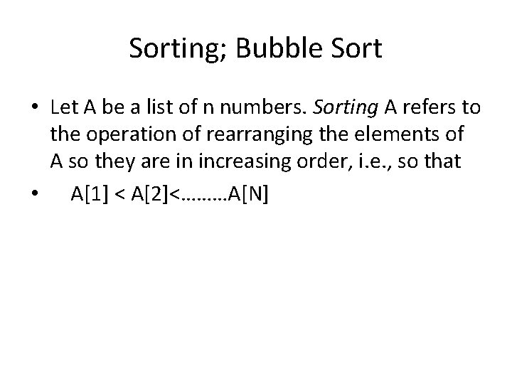
Sorting; Bubble Sort • Let A be a list of n numbers. Sorting A refers to the operation of rearranging the elements of A so they are in increasing order, i. e. , so that • A[1] < A[2]<………A[N]

How Bubble sort works? • Suppose the list of numbers A[1], A[2], …. . A[N] is in memory. • See page # 74 for detail.

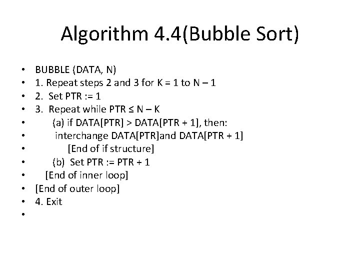
Algorithm 4. 4(Bubble Sort) • • • BUBBLE (DATA, N) 1. Repeat steps 2 and 3 for K = 1 to N – 1 2. Set PTR : = 1 3. Repeat while PTR ≤ N – K (a) if DATA[PTR] > DATA[PTR + 1], then: interchange DATA[PTR]and DATA[PTR + 1] [End of if structure] (b) Set PTR : = PTR + 1 [End of inner loop] [End of outer loop] 4. Exit

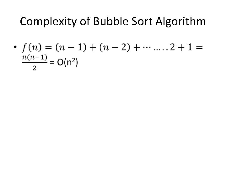
Complexity of Bubble Sort Algorithm •

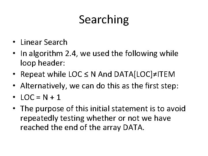
Searching • Linear Search • In algorithm 2. 4, we used the following while loop header: • Repeat while LOC ≤ N And DATA[LOC]≠ITEM • Alternatively, we can do this as the first step: • LOC = N + 1 • The purpose of this initial statement is to avoid repeatedly testing whether or not we have reached the end of the array DATA.

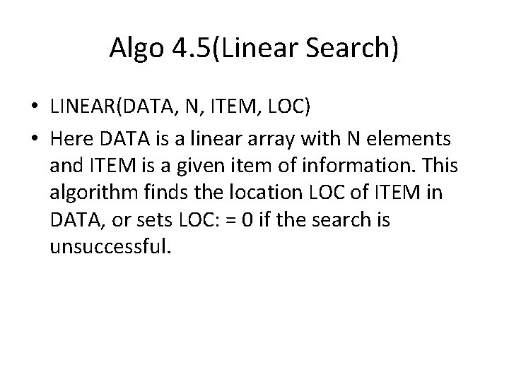
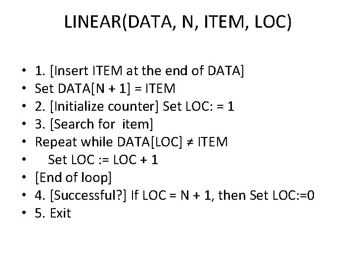
Algo 4. 5(Linear Search) • LINEAR(DATA, N, ITEM, LOC) • Here DATA is a linear array with N elements and ITEM is a given item of information. This algorithm finds the location LOC of ITEM in DATA, or sets LOC: = 0 if the search is unsuccessful.

LINEAR(DATA, N, ITEM, LOC) • • • 1. [Insert ITEM at the end of DATA] Set DATA[N + 1] = ITEM 2. [Initialize counter] Set LOC: = 1 3. [Search for item] Repeat while DATA[LOC] ≠ ITEM Set LOC : = LOC + 1 [End of loop] 4. [Successful? ] If LOC = N + 1, then Set LOC: =0 5. Exit

Complexity of Linear Search Algorithm • Discuss it yourself (also see page # 77)

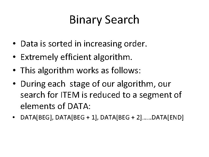
Binary Search • • Data is sorted in increasing order. Extremely efficient algorithm. This algorithm works as follows: During each stage of our algorithm, our search for ITEM is reduced to a segment of elements of DATA: • DATA[BEG], DATA[BEG + 1], DATA[BEG + 2]……DATA[END]

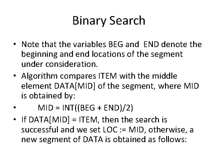
Binary Search • Note that the variables BEG and END denote the beginning and end locations of the segment under consideration. • Algorithm compares ITEM with the middle element DATA[MID] of the segment, where MID is obtained by: • MID = INT((BEG + END)/2) • If DATA[MID] = ITEM, then the search is successful and we set LOC : = MID, otherwise, a new segment of DATA is obtained as follows:

Binary Search • (a) If ITEM < DATA[MID], then ITEM can appear only in the left half of the segment: DATA[BEG], DATA[BEG + 1], DATA[BEG + 2]……DATA[MID - 1] So we reset END : = MID – 1 and begin searching again. • (b) If ITEM > DATA[MID], then ITEM can appear only in the right half of the segment: DATA[MID+1], DATA[MID + 2], ……DATA[END] So we reset BEG : = MID + 1 and begin searching again.

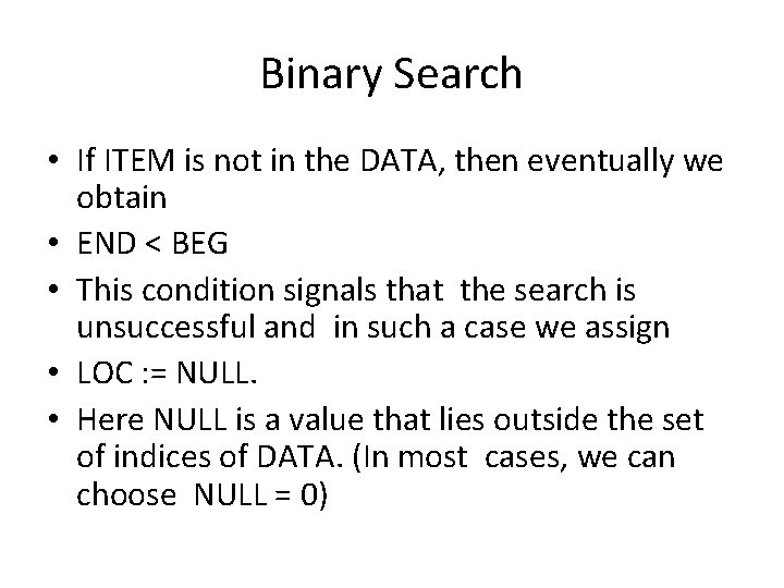
Binary Search • If ITEM is not in the DATA, then eventually we obtain • END < BEG • This condition signals that the search is unsuccessful and in such a case we assign • LOC : = NULL. • Here NULL is a value that lies outside the set of indices of DATA. (In most cases, we can choose NULL = 0)

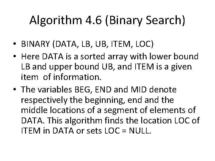
Algorithm 4. 6 (Binary Search) • BINARY (DATA, LB, UB, ITEM, LOC) • Here DATA is a sorted array with lower bound LB and upper bound UB, and ITEM is a given item of information. • The variables BEG, END and MID denote respectively the beginning, end and the middle locations of a segment of elements of DATA. This algorithm finds the location LOC of ITEM in DATA or sets LOC = NULL.

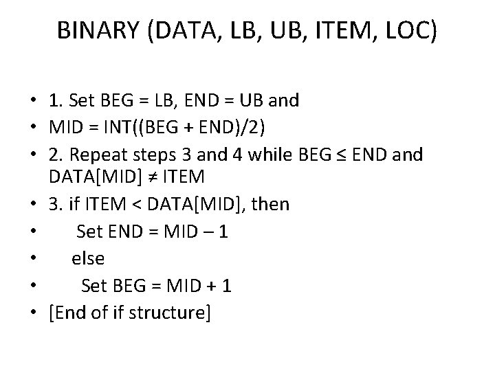
BINARY (DATA, LB, UB, ITEM, LOC) • 1. Set BEG = LB, END = UB and • MID = INT((BEG + END)/2) • 2. Repeat steps 3 and 4 while BEG ≤ END and DATA[MID] ≠ ITEM • 3. if ITEM < DATA[MID], then • Set END = MID – 1 • else • Set BEG = MID + 1 • [End of if structure]

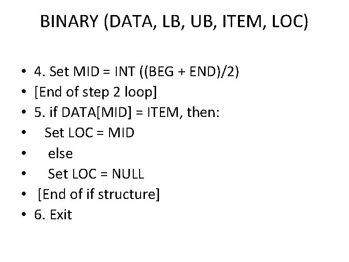
BINARY (DATA, LB, UB, ITEM, LOC) • • 4. Set MID = INT ((BEG + END)/2) [End of step 2 loop] 5. if DATA[MID] = ITEM, then: Set LOC = MID else Set LOC = NULL [End of if structure] 6. Exit

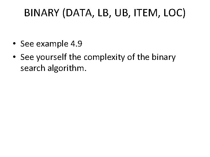
BINARY (DATA, LB, UB, ITEM, LOC) • See example 4. 9 • See yourself the complexity of the binary search algorithm.

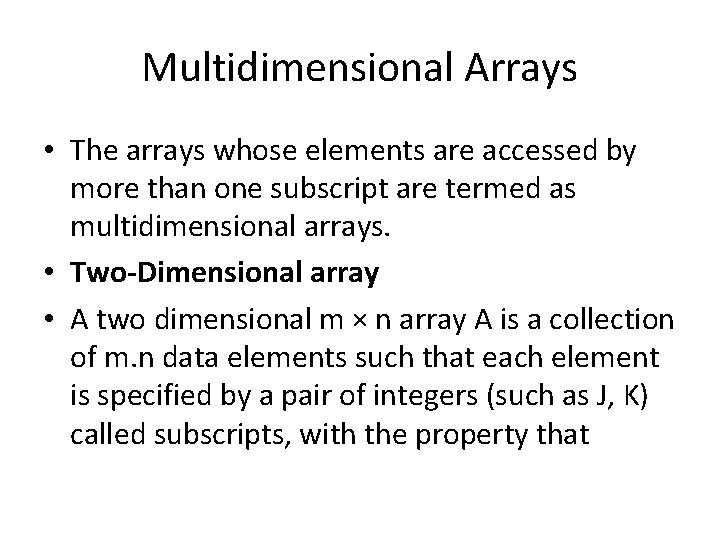
Multidimensional Arrays • The arrays whose elements are accessed by more than one subscript are termed as multidimensional arrays. • Two-Dimensional array • A two dimensional m × n array A is a collection of m. n data elements such that each element is specified by a pair of integers (such as J, K) called subscripts, with the property that

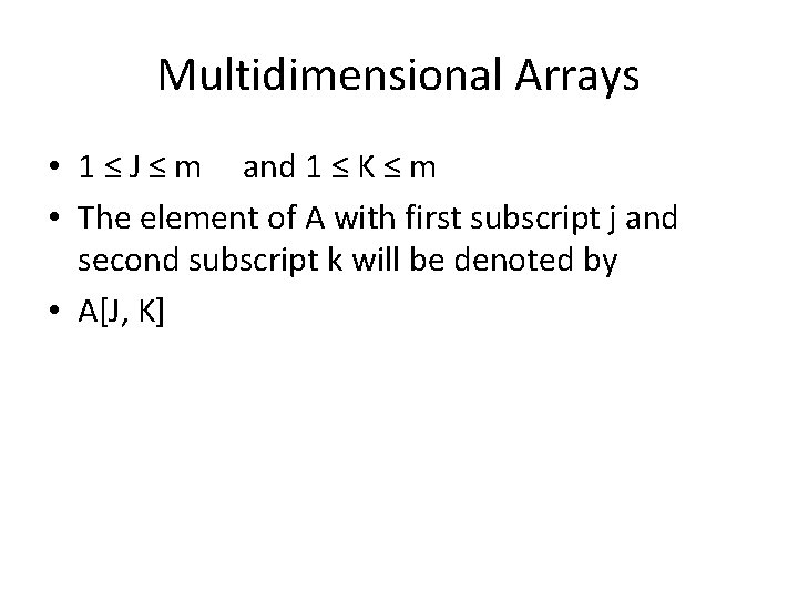
Multidimensional Arrays • 1 ≤ J ≤ m and 1 ≤ K ≤ m • The element of A with first subscript j and second subscript k will be denoted by • A[J, K]

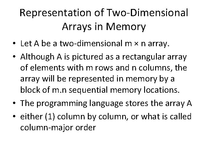
Representation of Two-Dimensional Arrays in Memory • Let A be a two-dimensional m × n array. • Although A is pictured as a rectangular array of elements with m rows and n columns, the array will be represented in memory by a block of m. n sequential memory locations. • The programming language stores the array A • either (1) column by column, or what is called column-major order

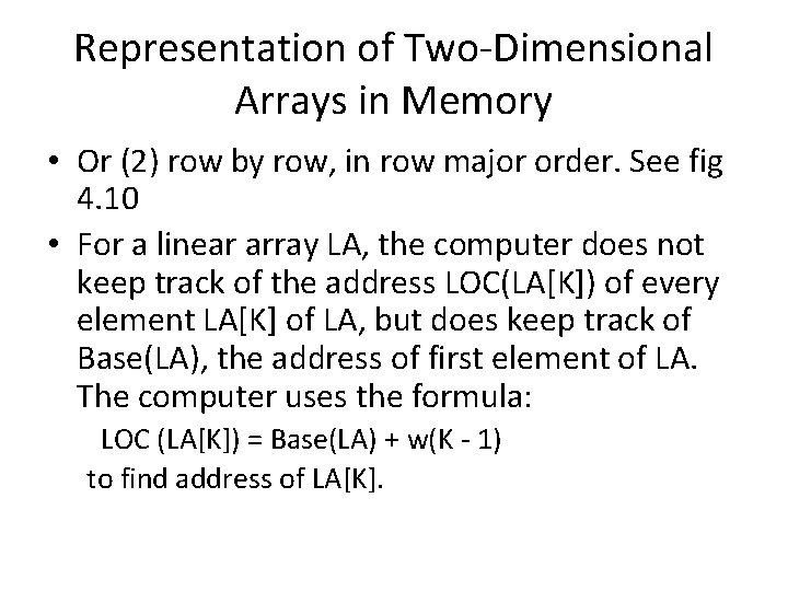
Representation of Two-Dimensional Arrays in Memory • Or (2) row by row, in row major order. See fig 4. 10 • For a linear array LA, the computer does not keep track of the address LOC(LA[K]) of every element LA[K] of LA, but does keep track of Base(LA), the address of first element of LA. The computer uses the formula: LOC (LA[K]) = Base(LA) + w(K - 1) to find address of LA[K].

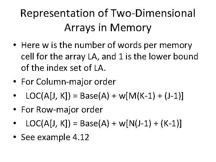
Representation of Two-Dimensional Arrays in Memory • Here w is the number of words per memory cell for the array LA, and 1 is the lower bound of the index set of LA. • For Column-major order • LOC(A[J, K]) = Base(A) + w[M(K-1) + (J-1)] • For Row-major order • LOC(A[J, K]) = Base(A) + w[N(J-1) + (K-1)] • See example 4. 12

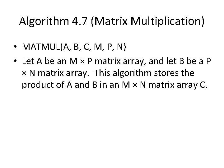
Algorithm 4. 7 (Matrix Multiplication) • MATMUL(A, B, C, M, P, N) • Let A be an M × P matrix array, and let B be a P × N matrix array. This algorithm stores the product of A and B in an M × N matrix array C.

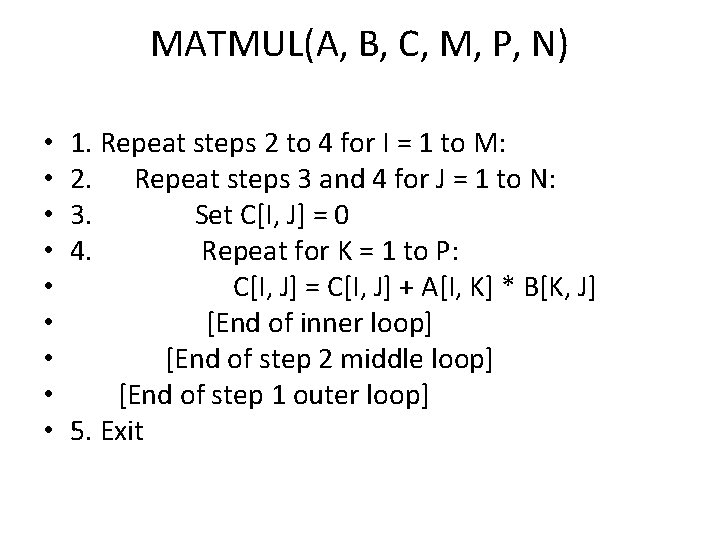
MATMUL(A, B, C, M, P, N) • • • 1. Repeat steps 2 to 4 for I = 1 to M: 2. Repeat steps 3 and 4 for J = 1 to N: 3. Set C[I, J] = 0 4. Repeat for K = 1 to P: C[I, J] = C[I, J] + A[I, K] * B[K, J] [End of inner loop] [End of step 2 middle loop] [End of step 1 outer loop] 5. Exit

SPARSE MATRICES • Matrices with relatively high proportion of zero entries are called sparse matrices.