Arrays 1 D Array Representation In C Memory

Arrays

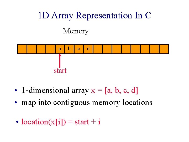
1 D Array Representation In C Memory a b c d start • 1 -dimensional array x = [a, b, c, d] • map into contiguous memory locations • location(x[i]) = start + i

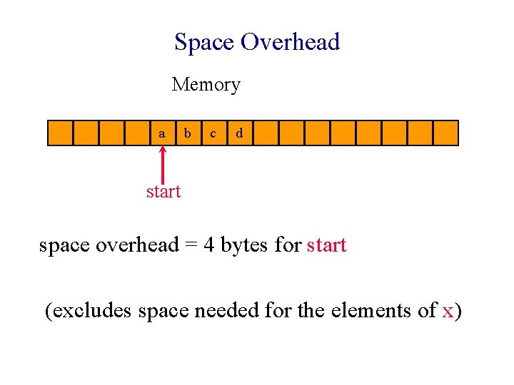
Space Overhead Memory a b c d start space overhead = 4 bytes for start (excludes space needed for the elements of x)

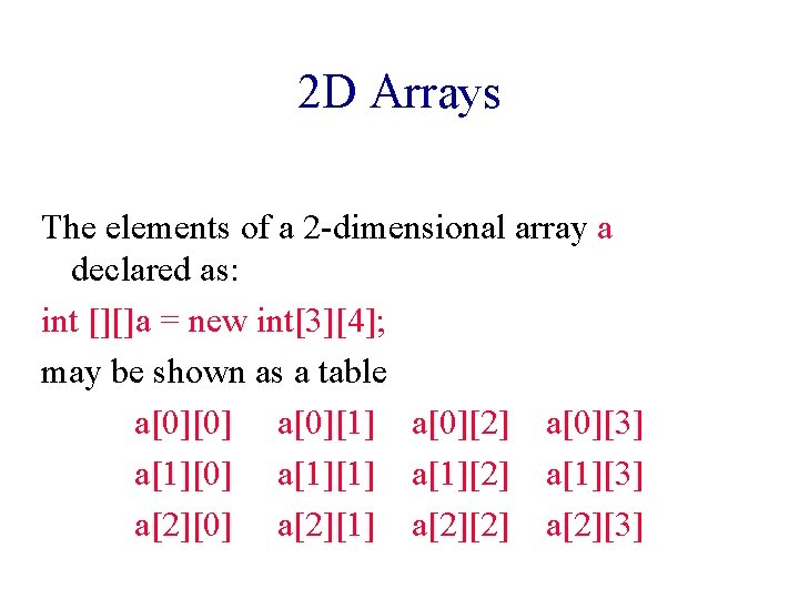
2 D Arrays The elements of a 2 -dimensional array a declared as: int [][]a = new int[3][4]; may be shown as a table a[0][0] a[0][1] a[0][2] a[0][3] a[1][0] a[1][1] a[1][2] a[1][3] a[2][0] a[2][1] a[2][2] a[2][3]

Rows Of A 2 D Array a[0][0] a[1][0] a[2][0] a[0][1] a[1][1] a[2][1] a[0][2] a[1][2] a[2][2] a[0][3] a[1][3] a[2][3] row 0 row 1 row 2

Columns Of A 2 D Array a[0][0] a[1][0] a[2][0] a[0][1] a[1][1] a[2][1] a[0][2] a[1][2] a[2][2] a[0][3] a[1][3] a[2][3] column 0 column 1 column 2 column 3

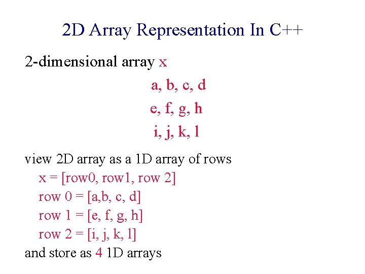
2 D Array Representation In C++ 2 -dimensional array x a, b, c, d e, f, g, h i, j, k, l view 2 D array as a 1 D array of rows x = [row 0, row 1, row 2] row 0 = [a, b, c, d] row 1 = [e, f, g, h] row 2 = [i, j, k, l] and store as 4 1 D arrays

2 D Array Representation In C x[] a b c d e f g h i j k l

Space Overhead x[] a b c d e f g h i j k l space overhead = space required by the array x[] = 3 * 4 bytes = 12 bytes = number of rows x 4 bytes

Array Representation In C x[] a b c d e f g h i j k l • This representation is called the array-of-arrays representation. • Requires contiguous memory of size 3, 4, 4, and 4 for the 4 1 D arrays. • 1 memory block of size number of rows and number of rows blocks of size number of columns

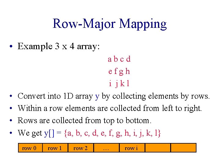
Row-Major Mapping • Example 3 x 4 array: • • abcd efgh i jkl Convert into 1 D array y by collecting elements by rows. Within a row elements are collected from left to right. Rows are collected from top to bottom. We get y[] = {a, b, c, d, e, f, g, h, i, j, k, l} row 0 row 1 row 2 … row i

Locating Element x[i][j] 0 c row 0 2 c row 1 • • • 3 c row 2 ic … row i assume x has r rows and c columns each row has c elements i rows to the left of row i so ic elements to the left of x[i][0] so x[i][j] is mapped to position ic + j of the 1 D array

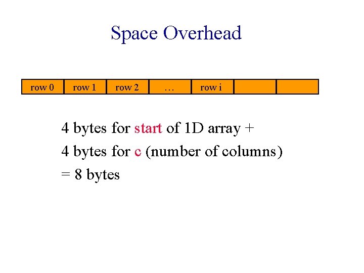
Space Overhead row 0 row 1 row 2 … row i 4 bytes for start of 1 D array + 4 bytes for c (number of columns) = 8 bytes

Disadvantage Need contiguous memory of size rc.

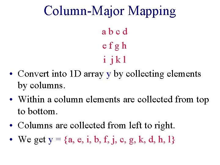
Column-Major Mapping • • abcd efgh i jkl Convert into 1 D array y by collecting elements by columns. Within a column elements are collected from top to bottom. Columns are collected from left to right. We get y = {a, e, i, b, f, j, c, g, k, d, h, l}

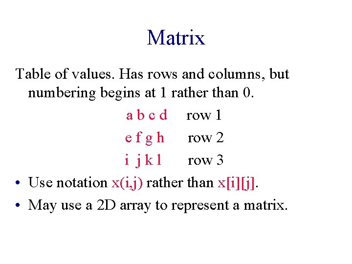
Matrix Table of values. Has rows and columns, but numbering begins at 1 rather than 0. a b c d row 1 efgh row 2 i jkl row 3 • Use notation x(i, j) rather than x[i][j]. • May use a 2 D array to represent a matrix.

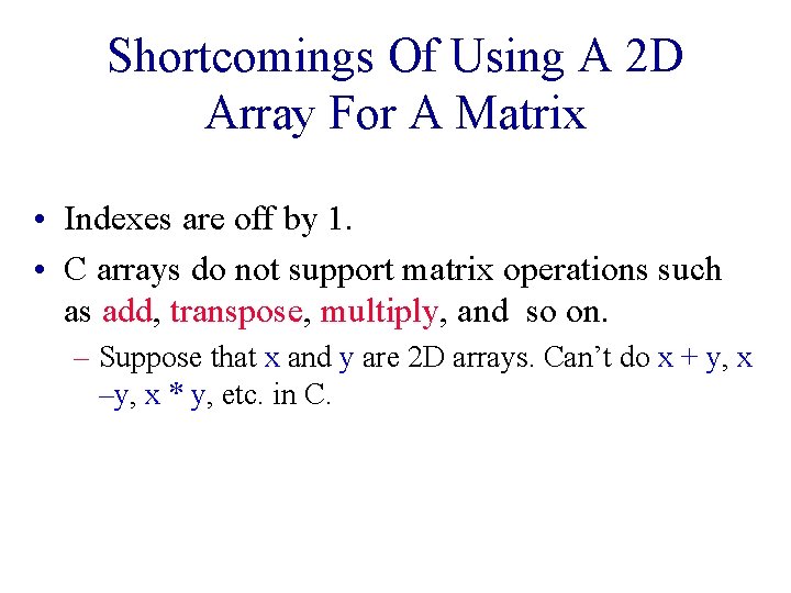
Shortcomings Of Using A 2 D Array For A Matrix • Indexes are off by 1. • C arrays do not support matrix operations such as add, transpose, multiply, and so on. – Suppose that x and y are 2 D arrays. Can’t do x + y, x –y, x * y, etc. in C.

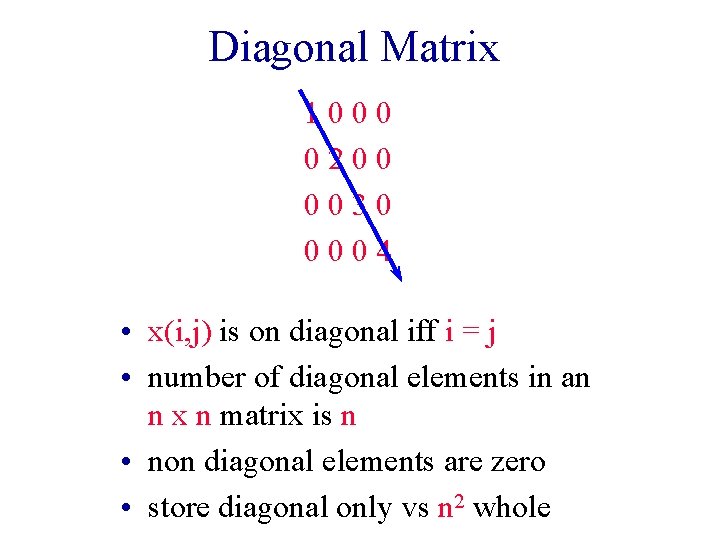
Diagonal Matrix An n x n matrix in which all nonzero terms are on the diagonal.

Diagonal Matrix 1000 0200 0030 0004 • x(i, j) is on diagonal iff i = j • number of diagonal elements in an n x n matrix is n • non diagonal elements are zero • store diagonal only vs n 2 whole

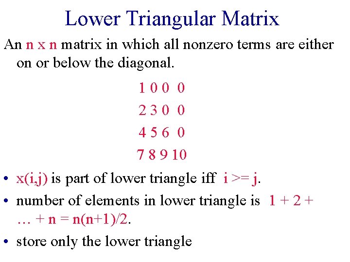
Lower Triangular Matrix An n x n matrix in which all nonzero terms are either on or below the diagonal. 100 0 230 0 456 0 7 8 9 10 • x(i, j) is part of lower triangle iff i >= j. • number of elements in lower triangle is 1 + 2 + … + n = n(n+1)/2. • store only the lower triangle

Array Of Arrays Representation x[] 1 2 3 4 5 6 7 8 9 l 0 Use an irregular 2 -D array … length of rows is not required to be the same.

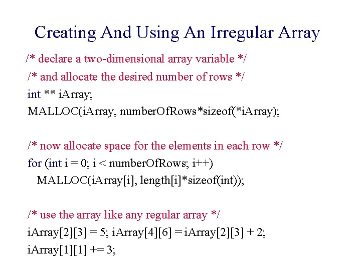
Creating And Using An Irregular Array /* declare a two-dimensional array variable */ /* and allocate the desired number of rows */ int ** i. Array; MALLOC(i. Array, number. Of. Rows*sizeof(*i. Array); /* now allocate space for the elements in each row */ for (int i = 0; i < number. Of. Rows; i++) MALLOC(i. Array[i], length[i]*sizeof(int)); /* use the array like any regular array */ i. Array[2][3] = 5; i. Array[4][6] = i. Array[2][3] + 2; i. Array[1][1] += 3;

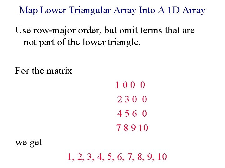
Map Lower Triangular Array Into A 1 D Array Use row-major order, but omit terms that are not part of the lower triangle. For the matrix 100 0 230 0 456 0 7 8 9 10 we get 1, 2, 3, 4, 5, 6, 7, 8, 9, 10

Index Of Element [i][j] 0 1 r 2 • • 3 6 r 3 … row i Order is: row 1, row 2, row 3, … Row i is preceded by rows 1, 2, …, i-1 Size of row i is i. Number of elements that precede row i is 1 + 2 + 3 + … + i-1 = i(i-1)/2 • So element (i, j) is at position i(i-1)/2 + j -1 of the 1 D array.