Arealization and Memory in the Cortex monkey Main

Arealization and Memory in the Cortex monkey Main perspectives: a) Hierarchical b) Modular c) Content-based

The hierarchical perspective The Elizabeth Gardner approach . . instead of neural activity (as in the Hopfield model). . ri = g[∑jwij. HEBBrj-Θ]+ wij . . do thermodynamics over connection weights, i. e. μ r consider whether among all i their possible values, there are which satisfy HEBB ≈ ∑ μ r i μr j μ = g[∑jwijrjμ-Θ]+

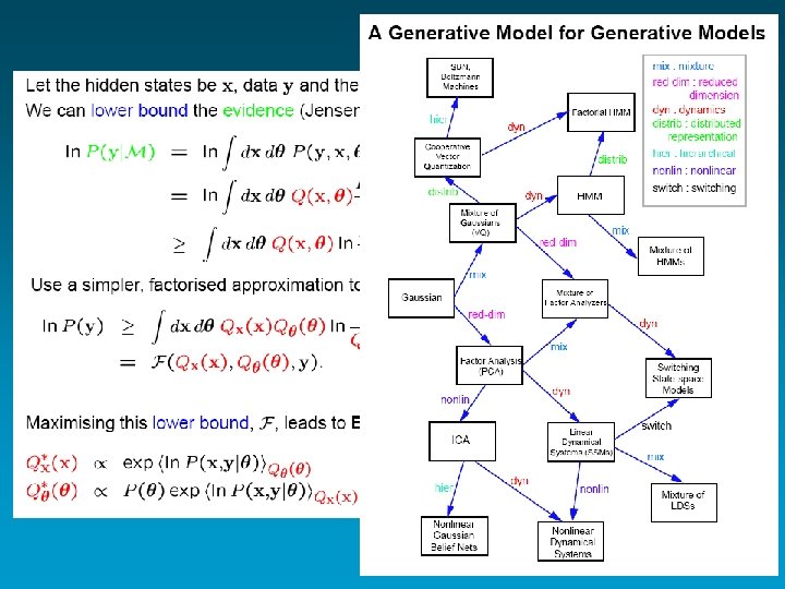
The hierarchical perspective The Elizabeth Gardner approach Backpropagation and E-M algorithms Network activation Forward Step: Δr Error propagation Backward Step: Δw Expectation – sampling the world Maximization – of the match between the world and our internal model of the world

The hierarchical perspective The Elizabeth Gardner approach Backpropagation and E-M algorithms Generative models paper by Hinton & Gharamani

The modular perspective The Braitenberg model N pyramidal cells √N compartments √N cells each A pical synapses B asal synapses

The modular perspective The Braitenberg model Modular associative memories Memory glass & capacity issues (with D O’Kane) Sparsity (with C Fulvi Mari) Latching dynamics (with E Kropff)

The modular perspective The Braitenberg model Modular associative memories Metricity in associative memory

slides of Anastasia Anishchenko (Brown) • Autoassociative memory retrieval is often studied using neural network models, in which connectivity does not follow any geometrical pattern, i. e. it is either all-to-all or, if sparse, randomly assigned – Storage capacity (max # patterns that can be retrieved) is proportional to the number k of connections per unit • Networks with a regular geometrical rule informing their connectivity, instead, often display geometrical patterns of activity, i. e. stabilize into activity profile `bumps` of width proportional to k • Recently, applications in various fields have used the fact that smallworld networks, characterized by a connectivity intermediate between regular and random, have different graph theoretic properties than either regular or random networks – Autoassociative memory retrieval? . . – Geometrical activity patterns? . . 9

CREATING A SMALL WORLD Watts, Strogatz 1998: • Start with a 1 D lattice ring • Rewire each edge at random with probability p • Rewiring of only a few edges is enough GRAPH THEORY DEFINITIONS • • • Graph consists of a nonempty set of elements, called vertices, and a list of unordered pairs of elements, called edges Order n of the graph = number of vertices Coordination number k = average number of edges connected to one vertex

PATH LENGTH and CLUSTERING • Characteristic path length L = length of the shortest path between two vertices, averaged over all pairs of vertices – L = average number of links in the shortest chain connecting two people x 0 x 1 x 2 x 3 L(x 0, x. M) = M x. M • Clustering coefficient C = average fraction of vertices linked. to one, which … are also linked to each other – All-to-all connectivity: C = 1 – Random connections: C = k / n << 1 for a large network

THREE DIFFERENT WORLDS • Regular: Cregular= C (0) ≈ ¾ Lregular= L (0) ≈ n/2 k SW LARGE • Random: C (p) ≈ C (0) L (p) ≈ L (1) small • Small World: Crandom= C (1) ≈ k/n LARGE Lrandom= L (1) ≈ ln(n)/ln(k) small REG RND Figure from Watts, Strogatz 1998

THE BRAIN IS A SMALL WORLD • Characteristic path length L and clustering coefficient C for cortex: § n = 1011 neurons, k = 104 connections per neuron § Lregular ≈ n / 2 k ≈ 107 synapses § Lrandom ≈ ln (n) / ln (k) ≈ 3 synapses too large realistic! But: § Crandom ≈ k/n ≈ 10 -7 too small • Cortex has short L (as random graph) and large C (as regular lattice) ðby definition, brain is a small world!. .

NETWORK MODEL • • N = 1000 neurons on a ring Integrate and fire: V 0 = -70 m. V, • – – Vthr= -54 m. V, m = 5 msec 1 = 30 msec, 2 = 4 msec, Connections: – – excitatory, all the same strength probabilistic Gaussian with a baseline: p global inhibition, inh = 4 msec drawn from a binary distribution (1 or 0) Sparseness = 0. 2 • Average number of connections per neuron k = 50 • Normalized modification of synaptic strength: • Give a cue for one of the patterns stored – “+” current into the “ 1” cells – – , • tref = 3 msec • Store M = 5 patterns • “-” current into the “ 0” cells Part of the cue may be randomly corrupted (partial cue)

CALCULATING L and C • Numerical results for L and C as functions of the parameter of randomness – Normalized and averaged over three network realizations • Analytical estimation of clustering coefficient: C = [1/sqrt(3) - k/n]*(1 -p)3 + k/n • Comparison with the numerical results (n = 1000, k = 50):

SPONTANEOUS ACTIVITY BUMPS Number of spikes • Nets with a regular geometrical rule guiding their connections (parameter of randomness p -> 0) often display geometrical patterns of activity, i. e. stabilize into activity profile "bumps“ – The width of the “bump” is proportional to number k of connections per neuron Neuron

ASSOCIATIVE MEMORY • Overlaps Oi , i = 1. . M of network activity with the M = 5 patterns stored before, during, & after a 75%-corrupted cue for pattern 2 was given – Samples taken for 50 msec every 50 msec during the simulation time cue

RETRIEVAL PERFORMANCE • Retrieval performance degrades gradually as the cue quality decreases • Memories can be retrieved with even when 90% of the cue input is corrupted

RETRIEVAL vs. “BUMPINESS” - I • The ability to retrieve memories dies if p 0. 4 – “prefers randomness” • The ability to form activity bumps dies if p 0. 6 – “prefers regularity” • Can they both be “alive enough” when 0. 4 < p < 0. 6 ? . .

Effect of changing cue size

RETRIEVAL vs. “BUMPINESS” - II • Increasing number k of connections per neuron. . . helps the memories. and interferes with the bumps • Changing k does not affect the qualitative picture, i. e. retrieval performance and bumpiness favor almost non -overlapping ranges of p • ”almost”: Is there still a chance for a successful coexistence at the same p? . .

RETRIEVAL vs. “BUMPINESS” - II • Increasing number k of connections per neuron. . . helps the memories. and interferes with the bumps • Changing k does not affect the qualitative picture, i. e. retrieval performance and bumpiness favor almost non -overlapping ranges of p • ”almost”: Is there still a chance for a successful coexistence at the same p? . .

CONCLUSIONS • The spontaneous activity bumps, which are formed in the regular network, can be observed up to p = 0. 6 • Storing random binary patterns in the network does not affect the bumps, but the retrieval performance appears to be very poor for small p • As the randomness increases (p > 0. 4), a robust retrieval is observed even for partial cues • Changing k does not affect the qualitative network behavior • The abilities to form stable activity bumps and to retrieve associative memories are favored at distinct ranges of the parameter of randomness – The “almost” question… Special thanks to the EU Advanced Course in Computational Neuroscience - Obidos, Portugal 2002 23

New CONCLUSIONS • Those were from Anastasia’s simulations • Enters Yasser with analytical calculations on a simpler (threshold-linear) model, supported by extensive simulations NEXT SLIDE

The content-based perspective An example: Plaut’s model of semantic memory . pdf