Arc Hydro Groundwater a geographic data model for

Arc Hydro Groundwater: a geographic data model for groundwater systems By Gil Strassberg, David Maidment and Norman Jones These slides are taken from the Ph. D Dissertation defense of Gil Strassberg in Nov 2005 Reference: http: //www. ce. utexas. edu/prof/maidment/giswr 2006/docs/strassberg. pdf We are discussing with ESRI the transformation of this work into an ESRI Press Book in 2007 This model won first prize for data models at the 2006 ESRI User Conference

Research questions 1. What are the primary hydrogeologic features common to groundwater studies in regional and site scales, and what is the best conceptual approach for describing them? 2. What are the basic features required for representing structures of groundwater simulation models, their inputs and outputs, and how can these structures be integrated within GIS? 3. What is the most efficient way to store, view, access, and analyze these features using current GIS technology? The data model design and implementation is the process through which these questions are answered

Outline 1. Introduction and data model goals 2. Arc Hydro groundwater data model design 3. Case studies (4 examples) 4. Conclusions

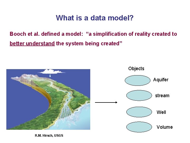
What is a data model? Booch et al. defined a model: “a simplification of reality created to better understand the system being created” Objects Aquifer stream Well Volume R. M. Hirsch, USGS

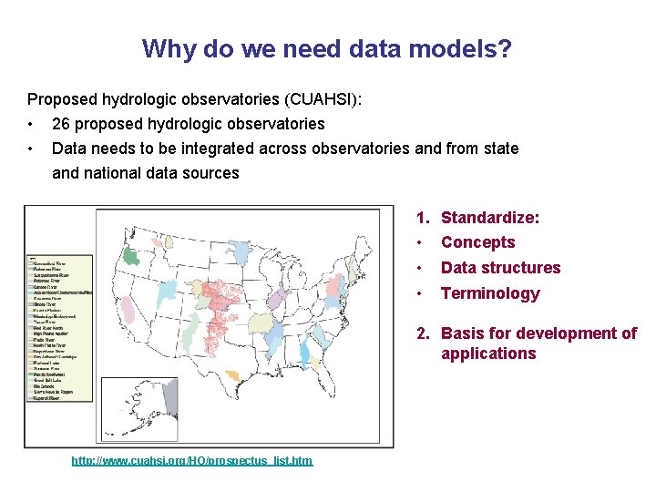
Why do we need data models? Proposed hydrologic observatories (CUAHSI): • • 26 proposed hydrologic observatories Data needs to be integrated across observatories and from state and national data sources 1. Standardize: • Concepts • Data structures • Terminology 2. Basis for development of applications http: //www. cuahsi. org/HO/prospectus_list. htm

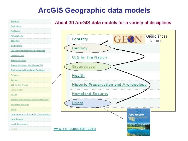
Arc. GIS Geographic data models About 30 Arc. GIS data models for a variety of disciplines Geosciences Network www. esri. com/datamodels

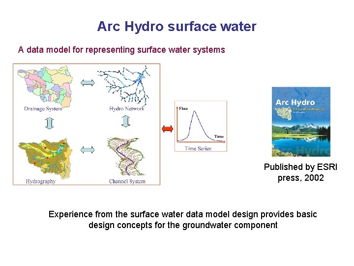
Arc Hydro surface water A data model for representing surface water systems Published by ESRI press, 2002 Experience from the surface water data model design provides basic design concepts for the groundwater component

Goals of the Arc Hydro groundwater data model Objective Develop a geographic data model for representing groundwater systems. Data model goals 1. Support representation of regional groundwater systems. 2. Support the representation of site scale groundwater data. 3. Enable the integration of surface water and groundwater data. 4. Facilitate the Integration of groundwater simulation models with GIS.

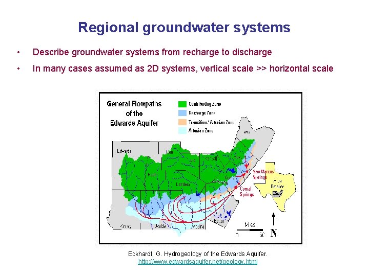
Regional groundwater systems • Describe groundwater systems from recharge to discharge • In many cases assumed as 2 D systems, vertical scale >> horizontal scale Eckhardt, G. Hydrogeology of the Edwards Aquifer. http: //www. edwardsaquifer. net/geology. html

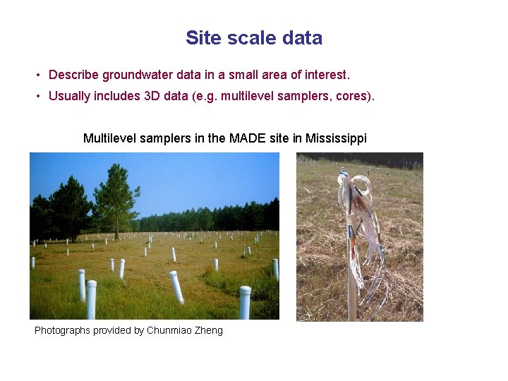
Site scale data • Describe groundwater data in a small area of interest. • Usually includes 3 D data (e. g. multilevel samplers, cores). Multilevel samplers in the MADE site in Mississippi Photographs provided by Chunmiao Zheng

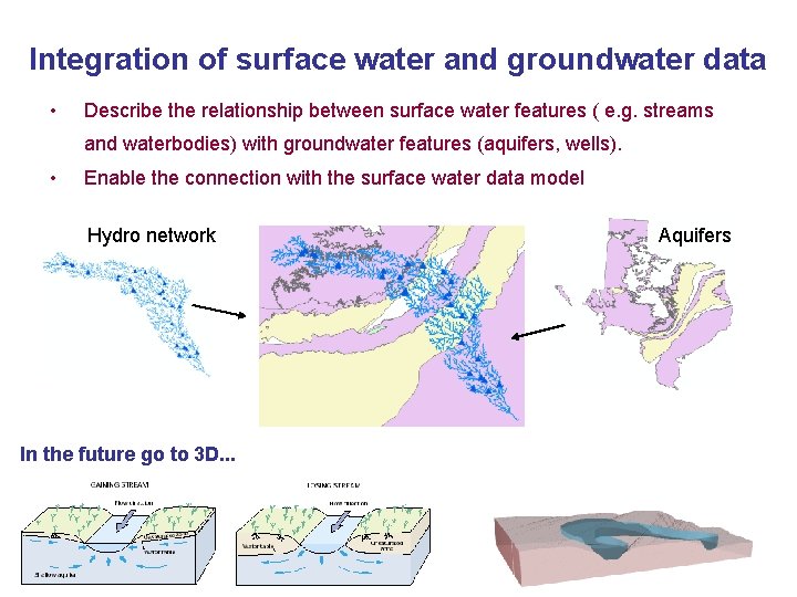
Integration of surface water and groundwater data • Describe the relationship between surface water features ( e. g. streams and waterbodies) with groundwater features (aquifers, wells). • Enable the connection with the surface water data model Hydro network In the future go to 3 D. . . Aquifers

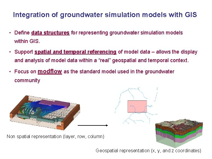
Integration of groundwater simulation models with GIS • Define data structures for representing groundwater simulation models within GIS. • Support spatial and temporal referencing of model data – allows the display and analysis of model data within a “real” geospatial and temporal context. • Focus on modflow as the standard model used in the groundwater community Non spatial representation (layer, row, column) Geospatial representation (x, y, and z coordinates)

Outline 1. Introduction and data model goals 2. Arc Hydro groundwater data model design 3. Case studies (4 examples) 4. Conclusions

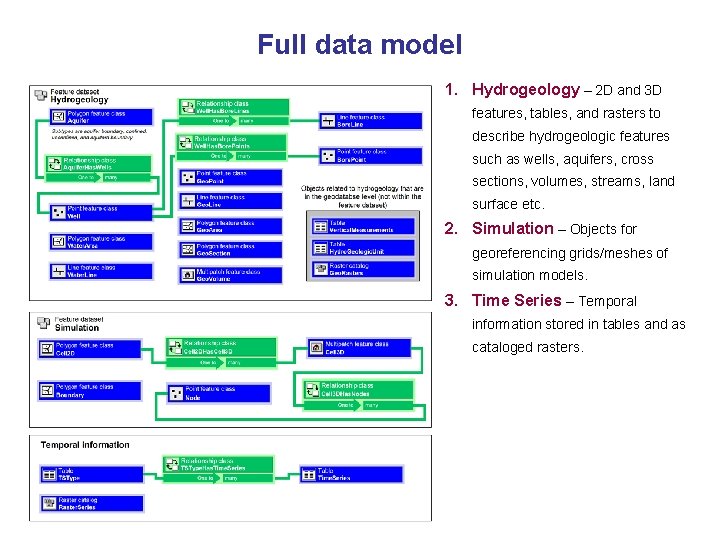
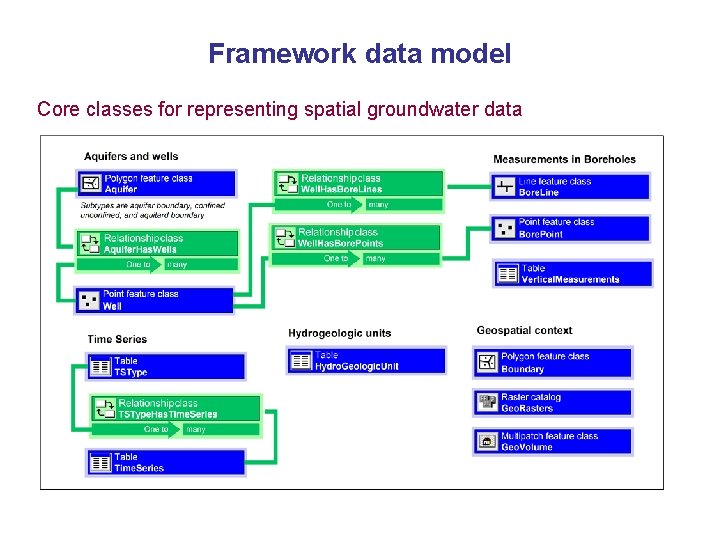
Full data model 1. Hydrogeology – 2 D and 3 D features, tables, and rasters to describe hydrogeologic features such as wells, aquifers, cross sections, volumes, streams, land surface etc. 2. Simulation – Objects for georeferencing grids/meshes of simulation models. 3. Time Series – Temporal information stored in tables and as cataloged rasters.

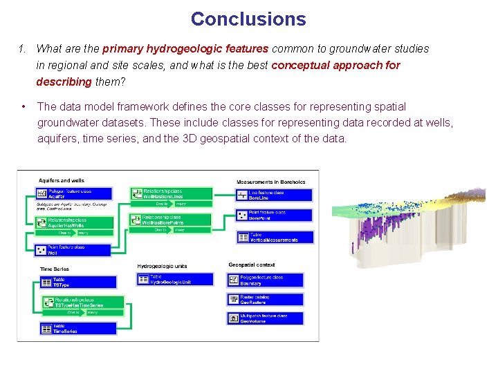
Framework data model Core classes for representing spatial groundwater data

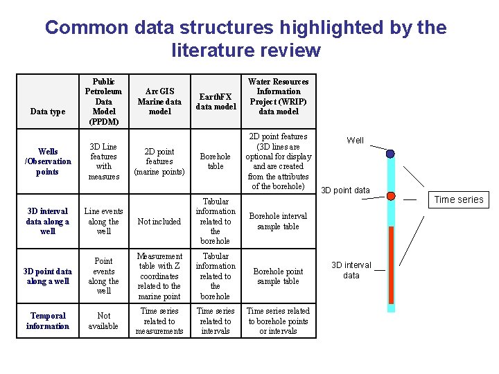
Common data structures highlighted by the literature review Data type Wells /Observation points Public Petroleum Data Model (PPDM) 3 D Line features with measures Arc. GIS Marine data model 2 D point features (marine points) Earth. FX data model Borehole table Water Resources Information Project (WRIP) data model 2 D point features (3 D lines are optional for display and are created from the attributes of the borehole) 3 D interval data along a well Line events along the well Not included Tabular information related to the borehole 3 D point data along a well Point events along the well Measurement table with Z coordinates related to the marine point Tabular information related to the borehole Borehole point sample table Temporal information Not available Time series related to measurements Time series related to intervals Time series related to borehole points or intervals Borehole interval sample table Well 3 D point data 3 D interval data Time series

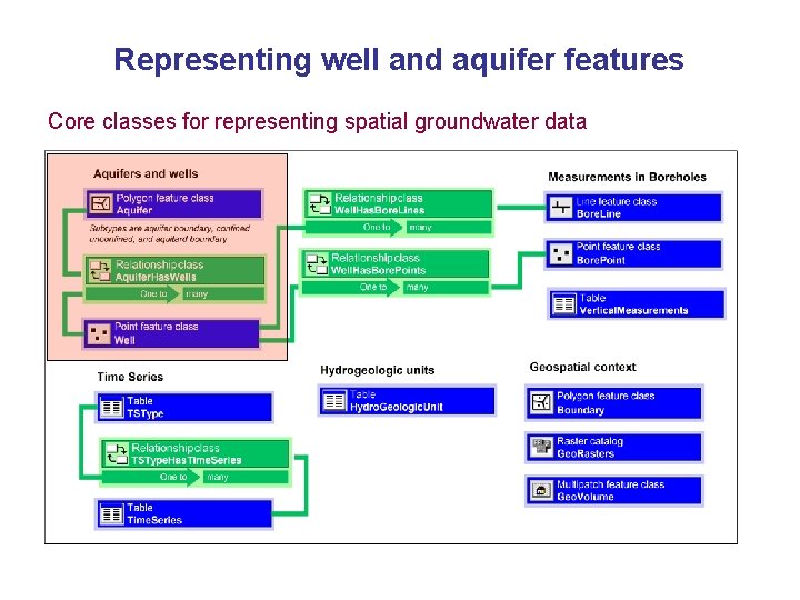
Representing well and aquifer features Core classes for representing spatial groundwater data

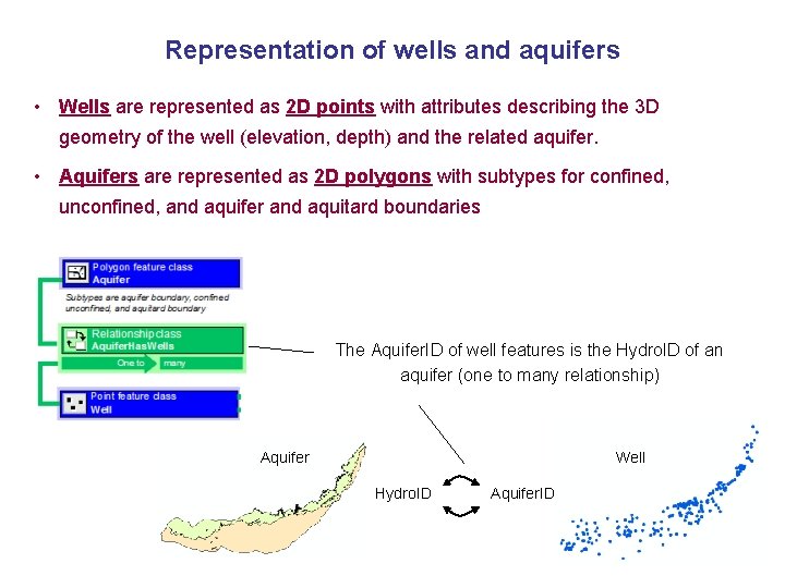
Representation of wells and aquifers • Wells are represented as 2 D points with attributes describing the 3 D geometry of the well (elevation, depth) and the related aquifer. • Aquifers are represented as 2 D polygons with subtypes for confined, unconfined, and aquifer and aquitard boundaries The Aquifer. ID of well features is the Hydro. ID of an aquifer (one to many relationship) Aquifer Well Hydro. ID Aquifer. ID

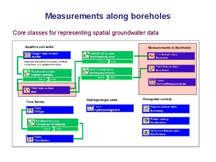
Measurements along boreholes Core classes for representing spatial groundwater data

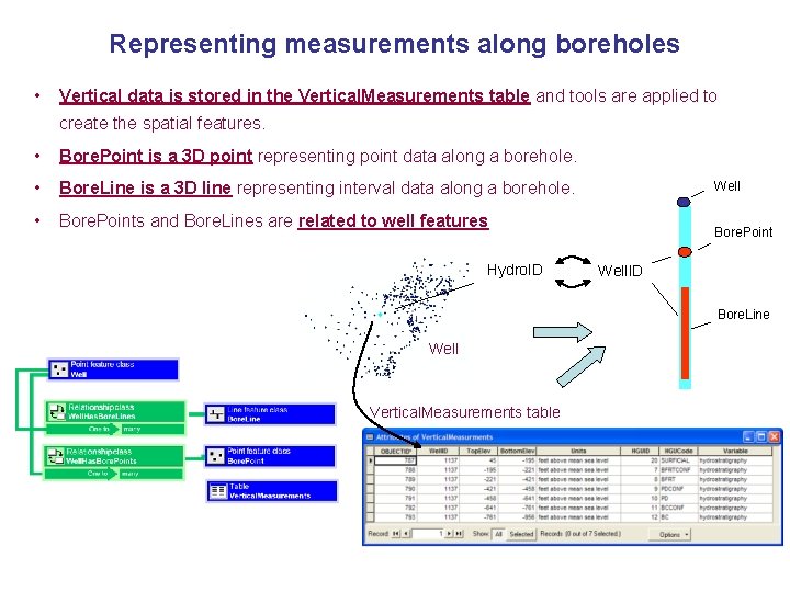
Representing measurements along boreholes • Vertical data is stored in the Vertical. Measurements table and tools are applied to create the spatial features. • Bore. Point is a 3 D point representing point data along a borehole. • Bore. Line is a 3 D line representing interval data along a borehole. • Bore. Points and Bore. Lines are related to well features Hydro. ID Well Bore. Point Well. ID Bore. Line Well Vertical. Measurements table

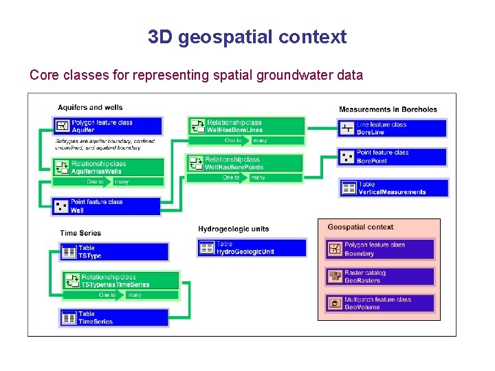
3 D geospatial context Core classes for representing spatial groundwater data

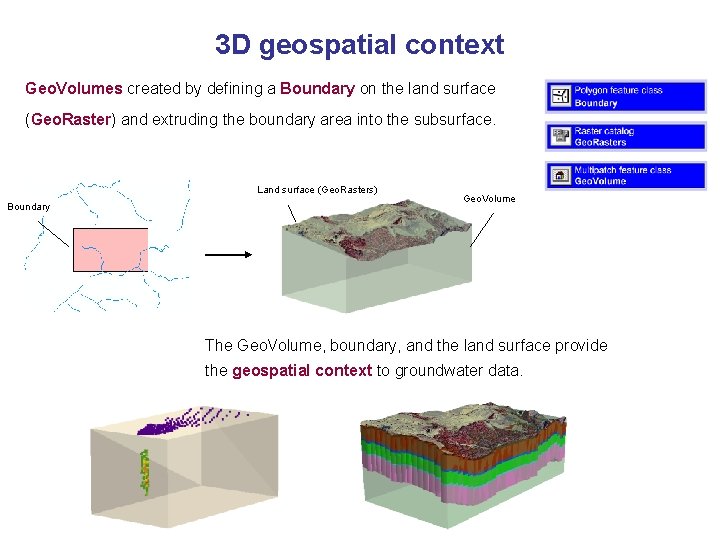
3 D geospatial context Geo. Volumes created by defining a Boundary on the land surface (Geo. Raster) and extruding the boundary area into the subsurface. Land surface (Geo. Rasters) Boundary Geo. Volume The Geo. Volume, boundary, and the land surface provide the geospatial context to groundwater data.

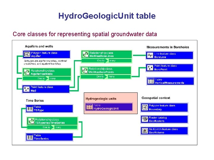
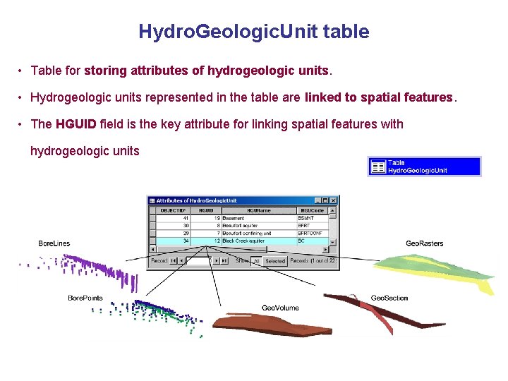
Hydro. Geologic. Unit table Core classes for representing spatial groundwater data

Hydro. Geologic. Unit table • Table for storing attributes of hydrogeologic units. • Hydrogeologic units represented in the table are linked to spatial features. • The HGUID field is the key attribute for linking spatial features with hydrogeologic units

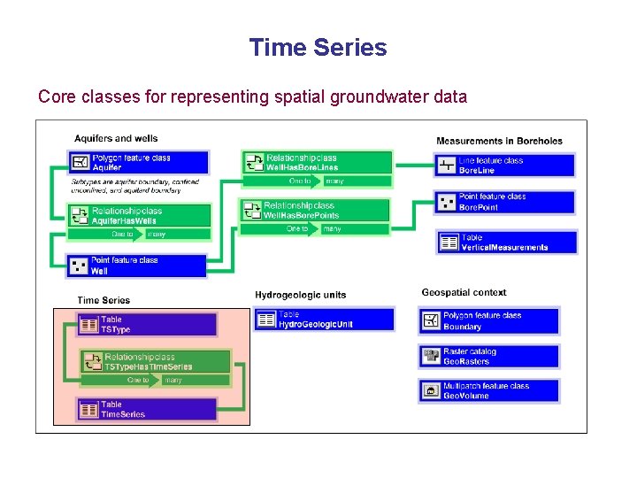
Time Series Core classes for representing spatial groundwater data

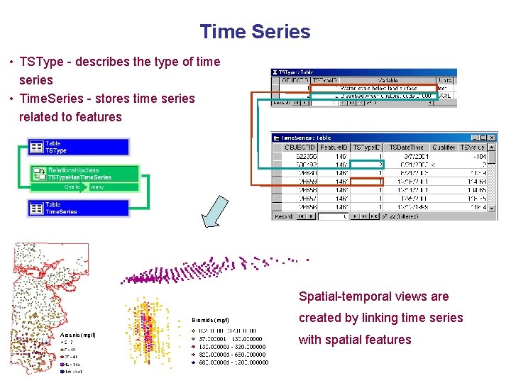
Time Series • TSType - describes the type of time series • Time. Series - stores time series related to features Spatial-temporal views are Bromide (mg/l) Arsenic (mg/l) created by linking time series with spatial features

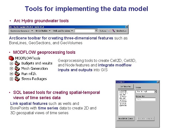
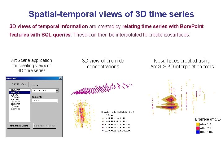
Tools for implementing the data model • Arc Hydro groundwater tools Arc. Scene toolbar for creating three-dimensional features such as Bore. Lines, Geo. Sections, and Geo. Volumes • MODFLOW geoprocessing tools Geoprocessing tools to create Cell 2 D, Cell 3 D, and Node features and integrate modflow inputs and outputs into GIS • SQL based tools for creating spatial-temporal views of time series data Link spatial features such as wells and Bore. Points with time series data to create 2 D and 3 D geospatial views of time series

Outline 1. Introduction and data model goals 2. Arc Hydro groundwater data model design 3. Case studies (4 examples) 4. Conclusions

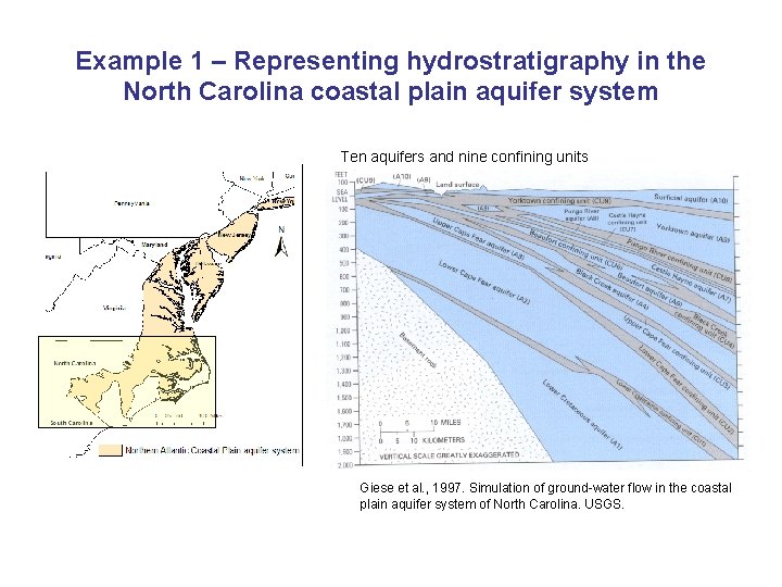
Example 1 – Representing hydrostratigraphy in the North Carolina coastal plain aquifer system Ten aquifers and nine confining units Giese et al. , 1997. Simulation of ground-water flow in the coastal plain aquifer system of North Carolina. USGS.

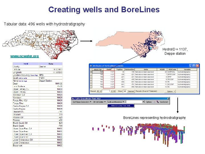
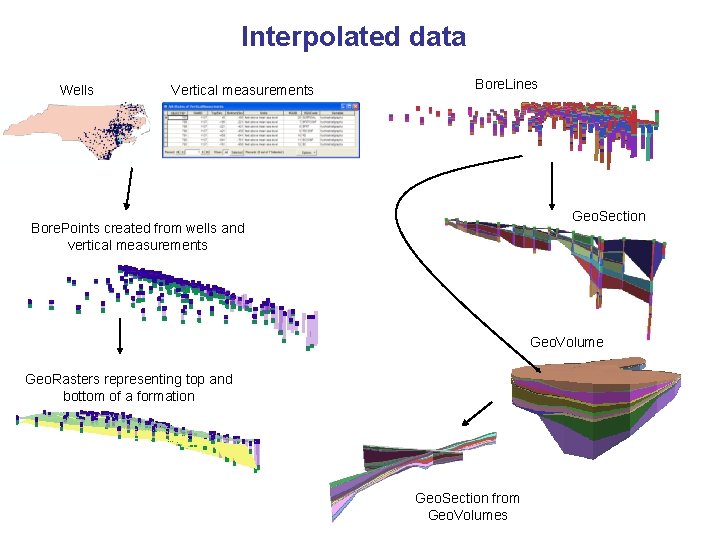
Creating wells and Bore. Lines Tabular data: 496 wells with hydrostratigraphy www. ncwater. org Hydro. ID = 1137, Deppe station Bore. Lines representing hydrostratigraphy

Interpolated data Wells Vertical measurements Bore. Lines Geo. Section Bore. Points created from wells and vertical measurements Geo. Volume Geo. Rasters representing top and bottom of a formation Geo. Section from Geo. Volumes

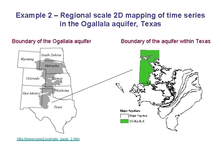
Example 2 – Regional scale 2 D mapping of time series in the Ogallala aquifer, Texas Boundary of the Ogallala aquifer http: //www. npwd. org/new_page_2. htm Boundary of the aquifer within Texas

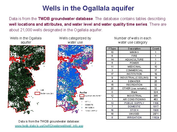
Wells in the Ogallala aquifer Data is from the TWDB groundwater database. The database contains tables describing well locations and attributes, and water level and water quality time series. There about 21, 000 wells designated in the Ogallala aquifer. Wells in the Ogallala aquifer Wells categorized by water use Number of wells in each water use category FType 10 6 14 5 11 3 17 9 4 15 20 0 12 1 13 7 16 18 8 Data is from the TWDB groundwater database: www. twdb. state. tx. us/Gw. RD/waterwell/well_info. asp Description MINING FIRE AQUACULTURE POWER MEDICINAL COMMERCIAL INSTITUTION INDUSTRIAL (COOLING) DEWATER RECREATION OTHER (see remarks) Blank INDUSTRIAL AIR CONDITIONING PUBLIC SUPPLY DOMESTIC STOCK UNUSED IRRIGATION Count 1 1 1 2 10 17 19 19 25 32 32 324 385 463 1106 1817 1928 2971 11824

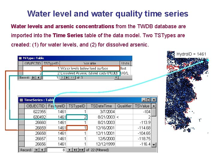
Water level and water quality time series Water levels and arsenic concentrations from the TWDB database are imported into the Time Series table of the data model. Two TSTypes are created: (1) for water levels, and (2) for dissolved arsenic. Hydro. ID = 1461

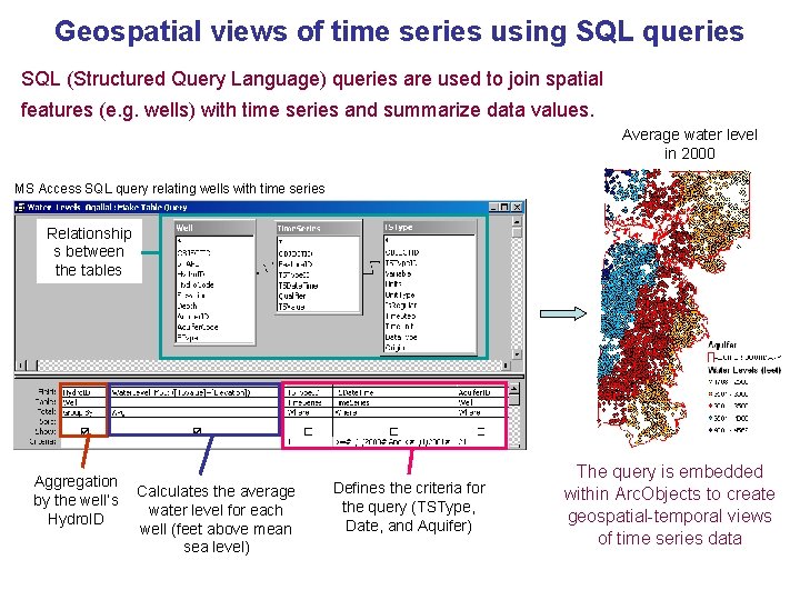
Geospatial views of time series using SQL queries SQL (Structured Query Language) queries are used to join spatial features (e. g. wells) with time series and summarize data values. Average water level in 2000 MS Access SQL query relating wells with time series Relationship s between the tables Aggregation by the well’s Hydro. ID Calculates the average water level for each well (feet above mean sea level) Defines the criteria for the query (TSType, Date, and Aquifer) The query is embedded within Arc. Objects to create geospatial-temporal views of time series data

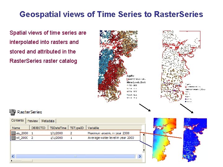
Geospatial views of Time Series to Raster. Series Spatial views of time series are interpolated into rasters and stored and attributed in the Raster. Series raster catalog

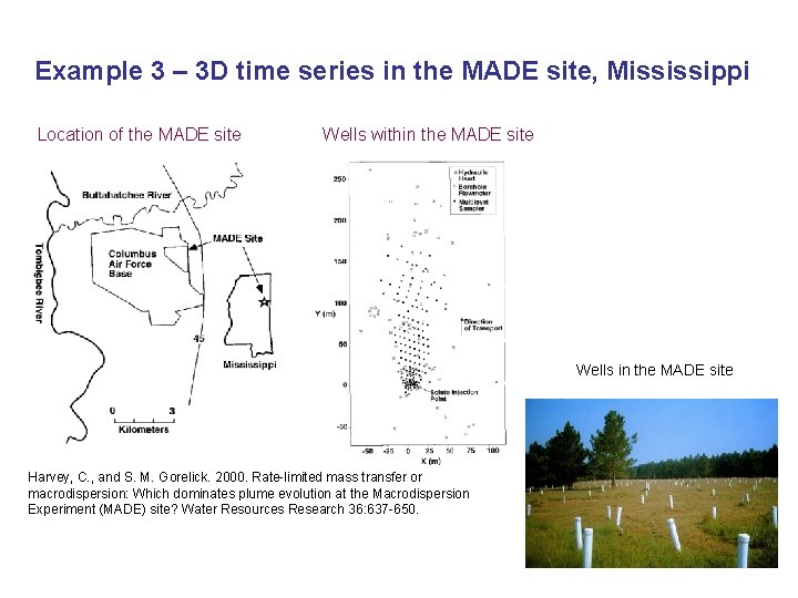
Example 3 – 3 D time series in the MADE site, Mississippi Location of the MADE site Wells within the MADE site Wells in the MADE site Harvey, C. , and S. M. Gorelick. 2000. Rate-limited mass transfer or macrodispersion: Which dominates plume evolution at the Macrodispersion Experiment (MADE) site? Water Resources Research 36: 637 -650.

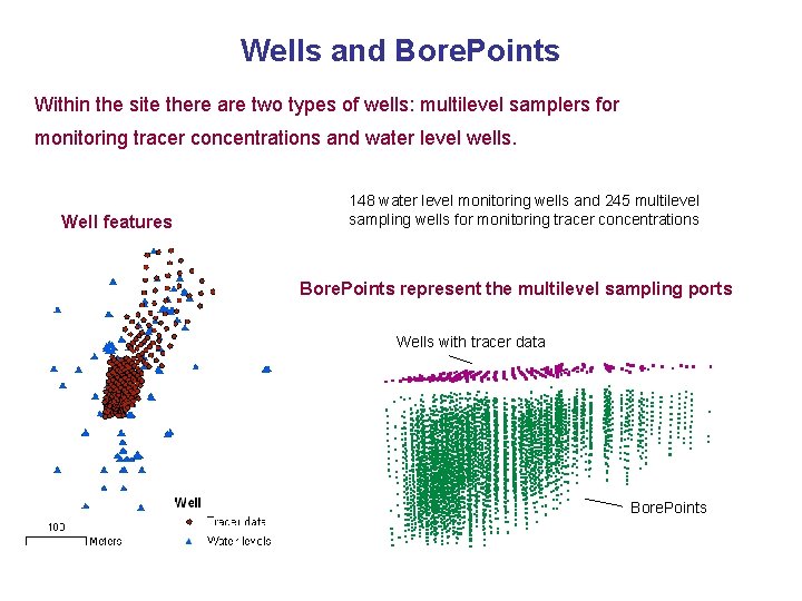
Wells and Bore. Points Within the site there are two types of wells: multilevel samplers for monitoring tracer concentrations and water level wells. Well features 148 water level monitoring wells and 245 multilevel sampling wells for monitoring tracer concentrations Bore. Points represent the multilevel sampling ports Wells with tracer data Bore. Points

Spatial-temporal views of 3 D time series 3 D views of temporal information are created by relating time series with Bore. Point features with SQL queries. These can then be interpolated to create isosurfaces. Arc. Scene application for creating views of 3 D time series 3 D view of bromide concentrations Isosurfaces created using Arc. GIS 3 D interpolation tools Bromide (mg/L)

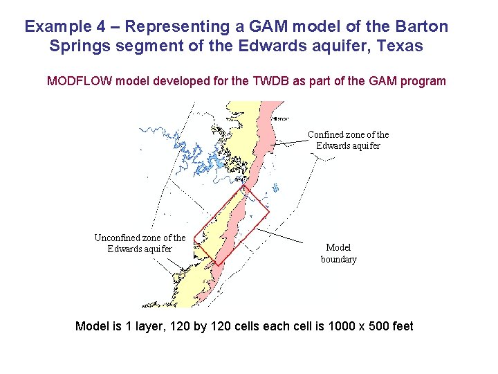
Example 4 – Representing a GAM model of the Barton Springs segment of the Edwards aquifer, Texas MODFLOW model developed for the TWDB as part of the GAM program Confined zone of the Edwards aquifer Unconfined zone of the Edwards aquifer Model boundary Model is 1 layer, 120 by 120 cells each cell is 1000 x 500 feet

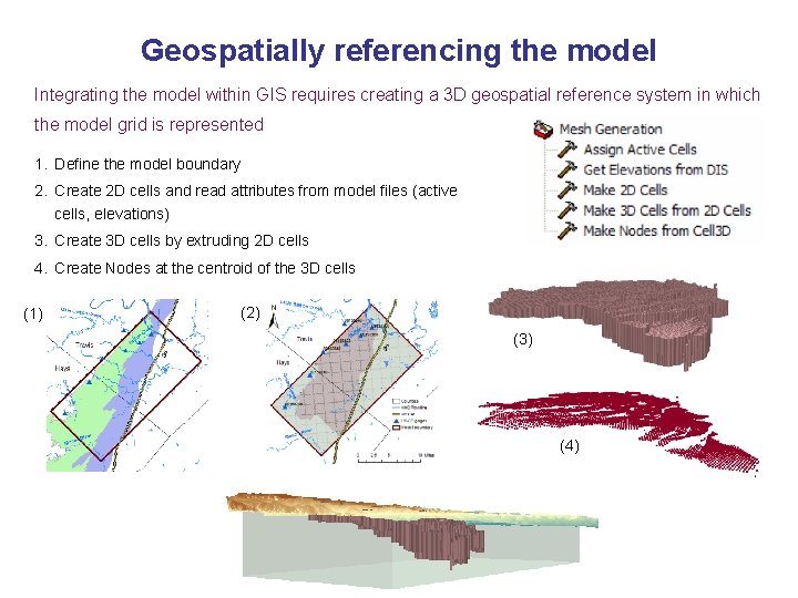
Geospatially referencing the model Integrating the model within GIS requires creating a 3 D geospatial reference system in which the model grid is represented 1. Define the model boundary 2. Create 2 D cells and read attributes from model files (active cells, elevations) 3. Create 3 D cells by extruding 2 D cells 4. Create Nodes at the centroid of the 3 D cells (1) (2) (3) (4)

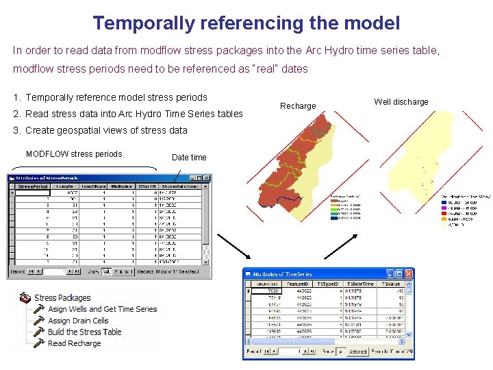
Temporally referencing the model In order to read data from modflow stress packages into the Arc Hydro time series table, modflow stress periods need to be referenced as “real” dates 1. Temporally reference model stress periods 2. Read stress data into Arc Hydro Time Series tables 3. Create geospatial views of stress data MODFLOW stress periods Date time Recharge Well discharge

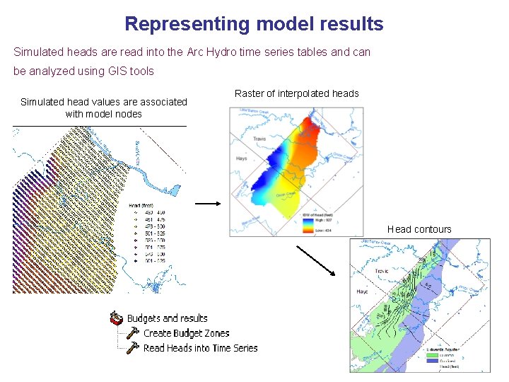
Representing model results Simulated heads are read into the Arc Hydro time series tables and can be analyzed using GIS tools Simulated head values are associated with model nodes Raster of interpolated heads Head contours

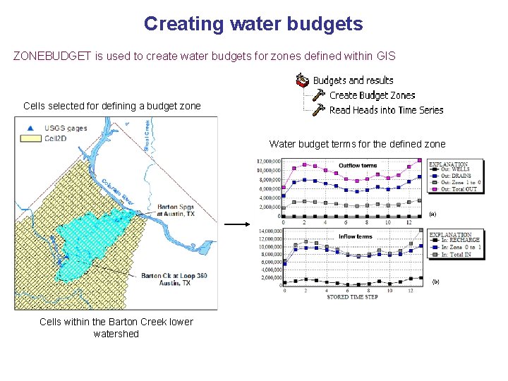
Creating water budgets ZONEBUDGET is used to create water budgets for zones defined within GIS Cells selected for defining a budget zone Water budget terms for the defined zone Cells within the Barton Creek lower watershed

Outline 1. Introduction and data model goals 2. Arc Hydro groundwater data model design (focus on the framework) 3. Case studies (4 examples) 4. Conclusions

Conclusions 1. What are the primary hydrogeologic features common to groundwater studies in regional and site scales, and what is the best conceptual approach for describing them? • The data model framework defines the core classes for representing spatial groundwater datasets. These include classes for representing data recorded at wells, aquifers, time series, and the 3 D geospatial context of the data.

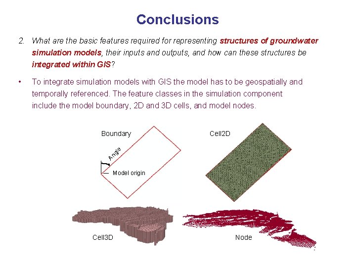
Conclusions 2. What are the basic features required for representing structures of groundwater simulation models, their inputs and outputs, and how can these structures be integrated within GIS? To integrate simulation models with GIS the model has to be geospatially and temporally referenced. The feature classes in the simulation component include the model boundary, 2 D and 3 D cells, and model nodes. Cell 2 D gl e Boundary An • Model origin Cell 3 D Node

Conclusions 3. What is the most efficient way to store, view, access, and analyze these features using current GIS technology? 3 D GIS • Combination of 2 D features and related tables, and 3 D features is most appropriate for managing 3 D information. • Time Series structures of Arc Hydro is appropriate for managing groundwater time series, and the combination with SQL queries is useful for creating spatialtemporal views of time series data. • Raster catalogs are useful to store, attribute, and index grids. Geo. Rasters are indexed by the HGUID to relate with a hydrogeologic unit, and Raster. Series are indexed by TSType and Date and Time. • XML is valuable for data exchange between applications