Arbitrage Pricing Theory and Multifactor Models Arbitrage Opportunity

Arbitrage Pricing Theory and Multifactor Models Arbitrage Opportunity and Profit Diversification and APT and CAPM Comparison Multifactor Models

Arbitrage Opportunity and Profit q Arbitrage Ø Ø q The opportunity of making riskless profit by exploiting relative mispricing of securities E. g. , IBM: $96 on NYSE and $96. 15 on NASDAQ creates an arbitrage opportunity Zero-Investment Portfolio Ø Ø A portfolio of zero value by long and short the same amount of securities E. g. , Buy $10, 000 of stock A and short $10, 000 of stock B creates a zero-investment portfolio Investments 12 2

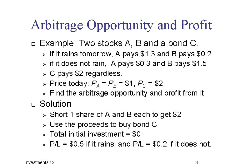
Arbitrage Opportunity and Profit q Example: Two stocks A, B and a bond C. Ø Ø Ø q If it rains tomorrow, A pays $1. 3 and B pays $0. 2 if it does not rain, A pays $0. 3 and B pays $1. 5 C pays $2 regardless. Price today: PA = PB = $1, PC = $2 Find the arbitrage opportunity and profit from it Solution Ø Ø Short 1 share of A and B each to get $2 Use the proceeds to buy bond C Total initial investment = $0 P/L = $0. 5 if it rains, and P/L = $0. 2 if it does not. Investments 12 3

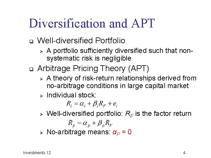
Diversification and APT q Well-diversified Portfolio Ø q A portfolio sufficiently diversified such that nonsystematic risk is negligible Arbitrage Pricing Theory (APT) Ø A theory of risk-return relationships derived from no-arbitrage conditions in large capital market Individual stock: Ø Well-diversified portfolio: RF is the factor return Ø No-arbitrage means: αP = 0 Ø Investments 12 4

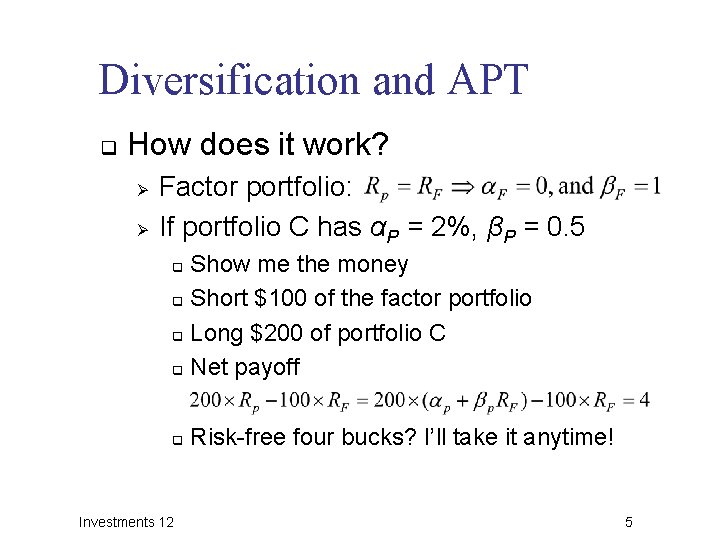
Diversification and APT q How does it work? Ø Ø Factor portfolio: If portfolio C has αP = 2%, βP = 0. 5 Show me the money q Short $100 of the factor portfolio q Long $200 of portfolio C q Net payoff q q Investments 12 Risk-free four bucks? I’ll take it anytime! 5

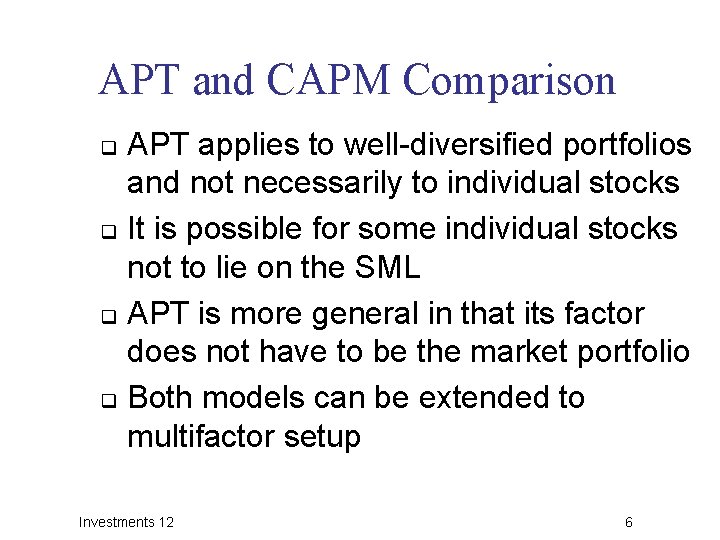
APT and CAPM Comparison APT applies to well-diversified portfolios and not necessarily to individual stocks q It is possible for some individual stocks not to lie on the SML q APT is more general in that its factor does not have to be the market portfolio q Both models can be extended to multifactor setup q Investments 12 6

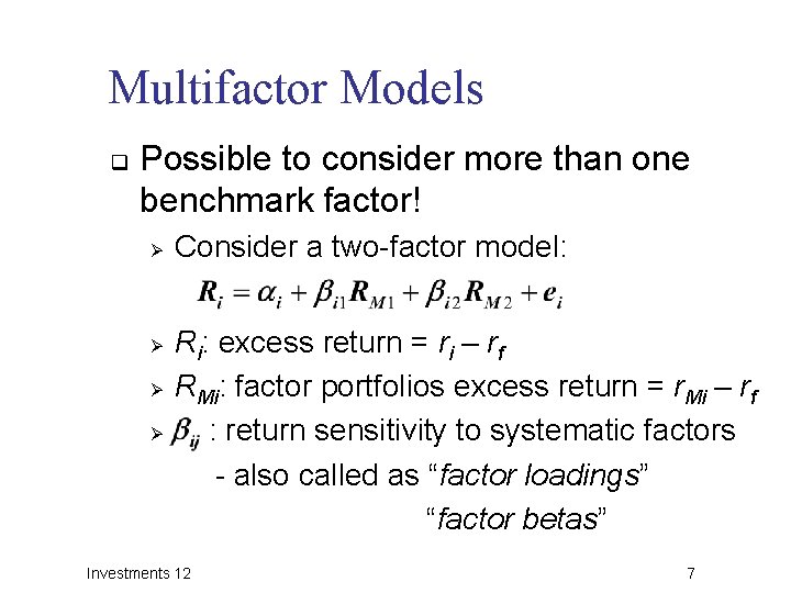
Multifactor Models q Possible to consider more than one benchmark factor! Ø Ø Consider a two-factor model: Ri: excess return = ri – rf RMi: factor portfolios excess return = r. Mi – rf : return sensitivity to systematic factors - also called as “factor loadings” “factor betas” Investments 12 7

Multifactor Models q Where do the factors come from? Ø Variables that reflect macroeconomic picture q Ø E. g. industrial production, inflation, bond spreads Variables that serve as proxies for exposure to systematic risk q Investments 12 E. g. Fama-French (1993) model approach 8

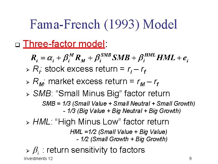
Fama-French (1993) Model q Three-factor model: Ø Ø Ø Ri: stock excess return = ri – rf RM: market excess return = r. M – rf SMB: “Small Minus Big” factor return SMB = 1/3 (Small Value + Small Neutral + Small Growth) - 1/3 (Big Value + Big Neutral + Big Growth) Ø HML: “High Minus Low” factor return HML =1/2 (Small Value + Big Value) - 1/2 (Small Growth + Big Growth) Ø : return sensitivity to factors Investments 12 9

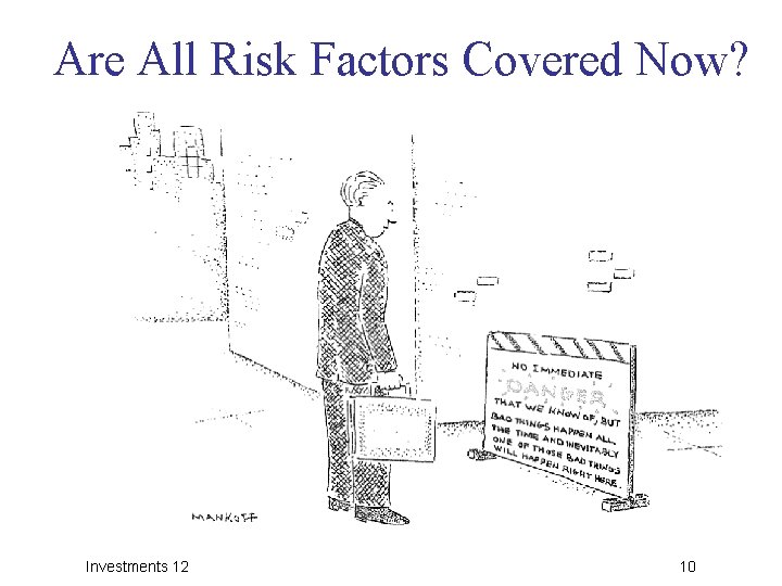
Are All Risk Factors Covered Now? Investments 12 10

Wrap-up What is arbitrage and how to do it? q What are the major differences between APT and CAPM? q Multifactor models – the way to go! q Investments 12 11