Approximation Algorithm Iterative Rounding Lecture 15 March 9

Approximation Algorithm: Iterative Rounding Lecture 15: March 9

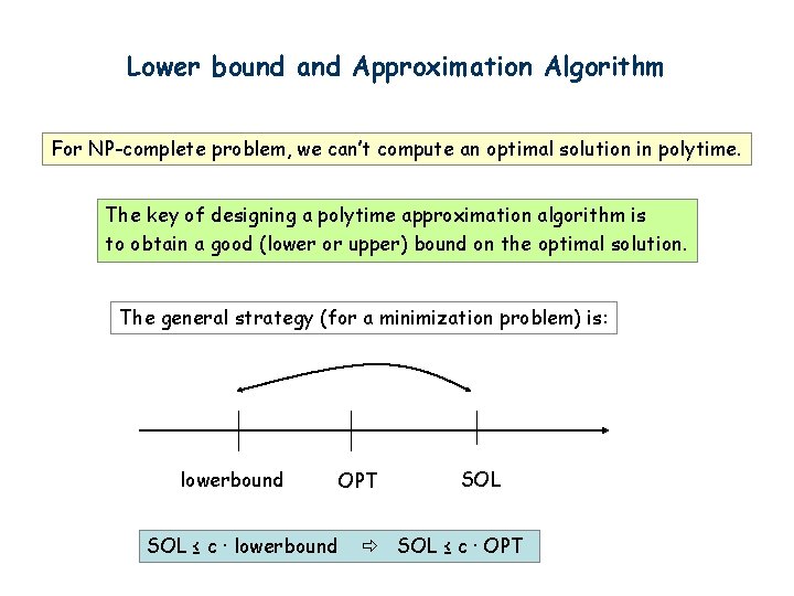
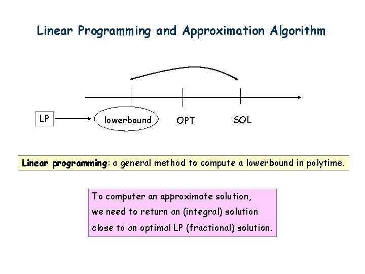
Lower bound and Approximation Algorithm For NP-complete problem, we can’t compute an optimal solution in polytime. The key of designing a polytime approximation algorithm is to obtain a good (lower or upper) bound on the optimal solution. The general strategy (for a minimization problem) is: lowerbound SOL ≤ c · lowerbound OPT SOL ≤ c · OPT

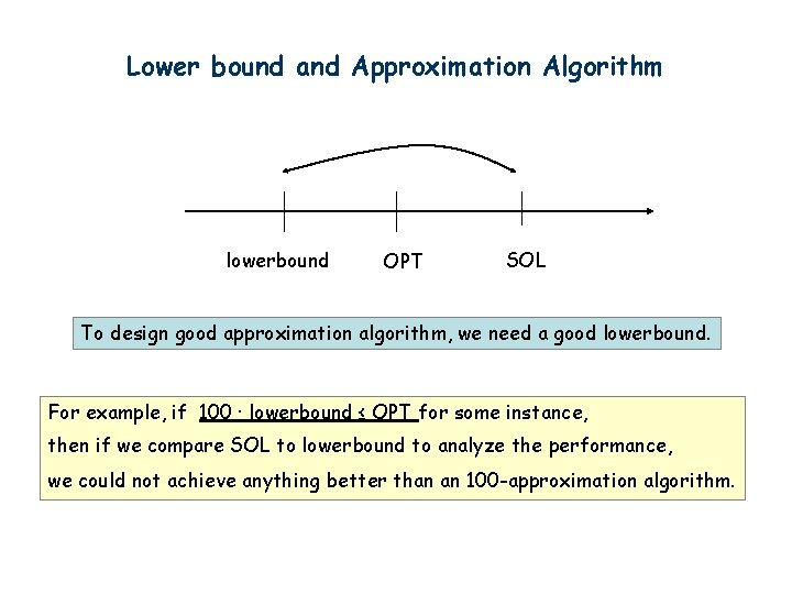
Lower bound and Approximation Algorithm lowerbound OPT SOL To design good approximation algorithm, we need a good lowerbound. For example, if 100 · lowerbound ≤ OPT for some instance, then if we compare SOL to lowerbound to analyze the performance, we could not achieve anything better than an 100 -approximation algorithm.

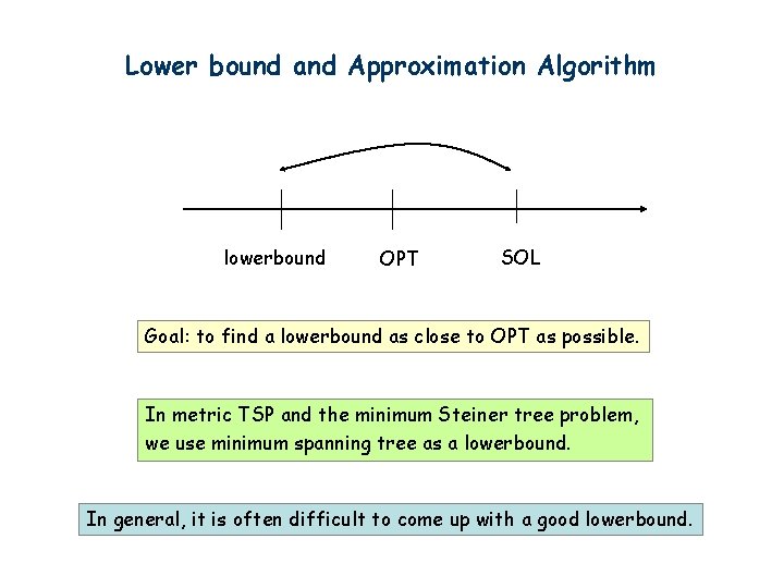
Lower bound and Approximation Algorithm lowerbound OPT SOL Goal: to find a lowerbound as close to OPT as possible. In metric TSP and the minimum Steiner tree problem, we use minimum spanning tree as a lowerbound. In general, it is often difficult to come up with a good lowerbound.

Linear Programming and Approximation Algorithm LP lowerbound OPT SOL Linear programming: a general method to compute a lowerbound in polytime. To computer an approximate solution, we need to return an (integral) solution close to an optimal LP (fractional) solution.

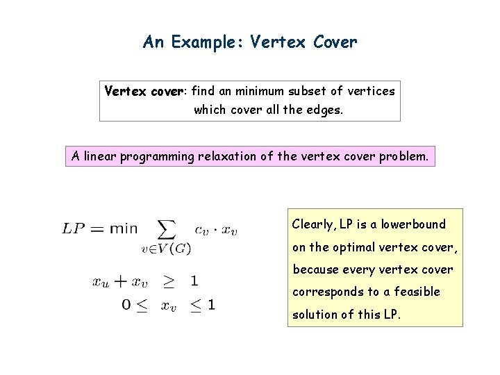
An Example: Vertex Cover Vertex cover: find an minimum subset of vertices which cover all the edges. A linear programming relaxation of the vertex cover problem. Clearly, LP is a lowerbound on the optimal vertex cover, because every vertex cover corresponds to a feasible solution of this LP.

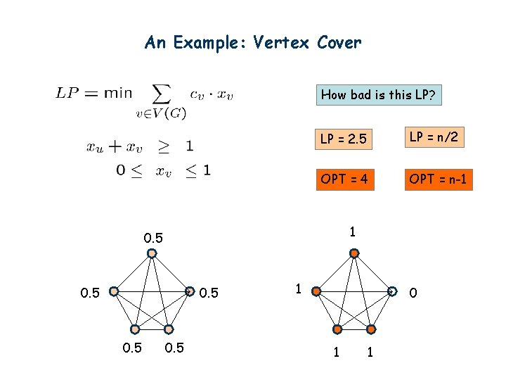
An Example: Vertex Cover How bad is this LP? LP = 2. 5 LP = n/2 OPT = 4 OPT = n-1 1 0. 5 0. 5 1 0 1 1

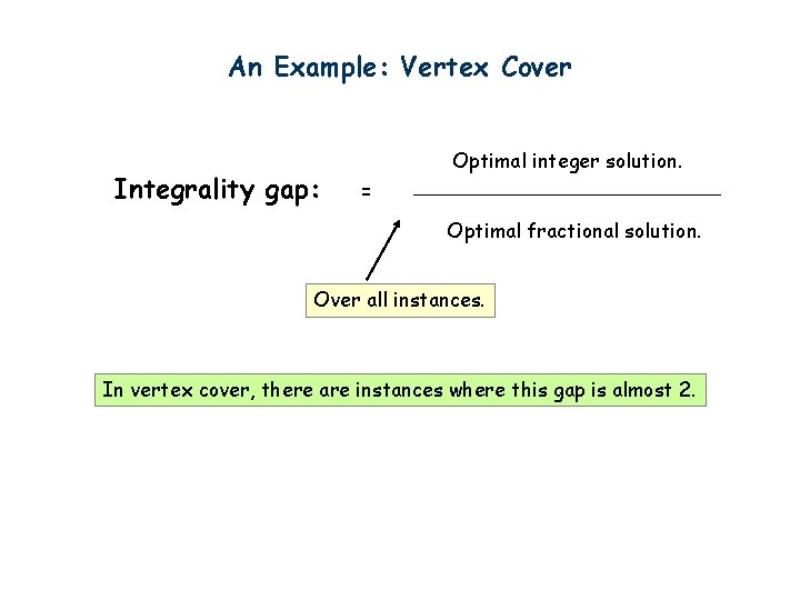
An Example: Vertex Cover Integrality gap: Optimal integer solution. = Optimal fractional solution. Over all instances. In vertex cover, there are instances where this gap is almost 2.

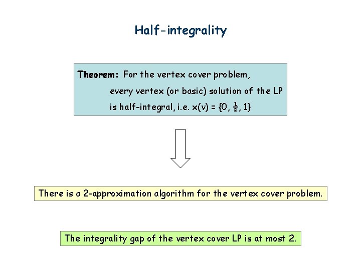
Half-integrality Theorem: For the vertex cover problem, every vertex (or basic) solution of the LP is half-integral, i. e. x(v) = {0, ½, 1} There is a 2 -approximation algorithm for the vertex cover problem. The integrality gap of the vertex cover LP is at most 2.

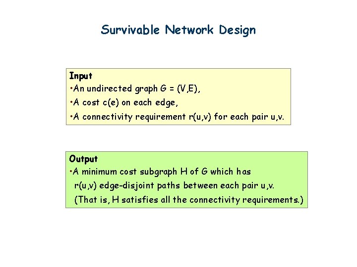
Survivable Network Design Input • An undirected graph G = (V, E), • A cost c(e) on each edge, • A connectivity requirement r(u, v) for each pair u, v. Output • A minimum cost subgraph H of G which has r(u, v) edge-disjoint paths between each pair u, v. (That is, H satisfies all the connectivity requirements. )

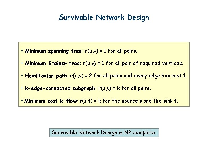
Survivable Network Design • Minimum spanning tree: r(u, v) = 1 for all pairs. • Minimum Steiner tree: r(u, v) = 1 for all pair of required vertices. • Hamiltonian path: r(u, v) = 2 for all pairs and every edge has cost 1. • k-edge-connected subgraph: r(u, v) = k for all pairs. • Minimum cost k-flow: r(s, t) = k for the source s and the sink t. Survivable Network Design is NP-complete.

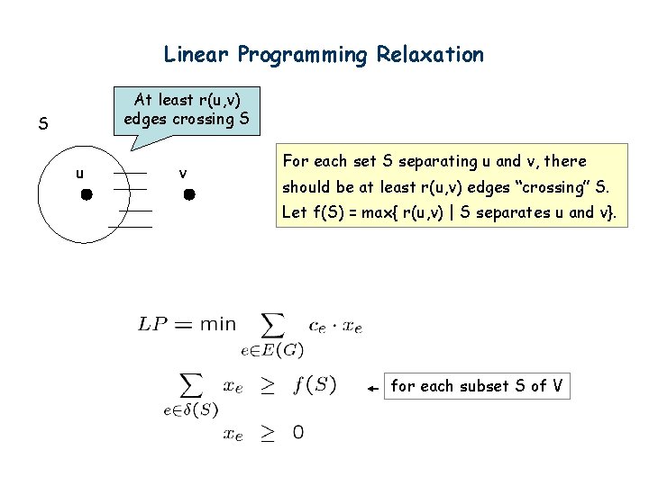
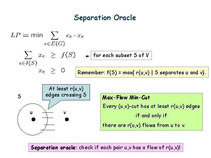
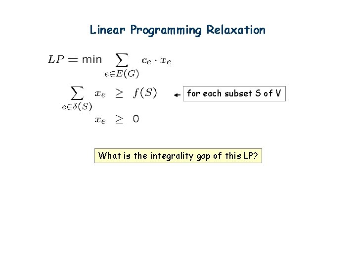
Linear Programming Relaxation At least r(u, v) edges crossing S S u v For each set S separating u and v, there should be at least r(u, v) edges “crossing” S. Let f(S) = max{ r(u, v) | S separates u and v}. for each subset S of V

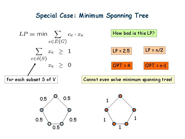
Special Case: Minimum Spanning Tree How bad is this LP? for each subset S of V 0. 5 LP = n/2 OPT = 4 OPT = n-1 Cannot even solve minimum spanning tree! 0. 5 LP = 2. 5 1 1

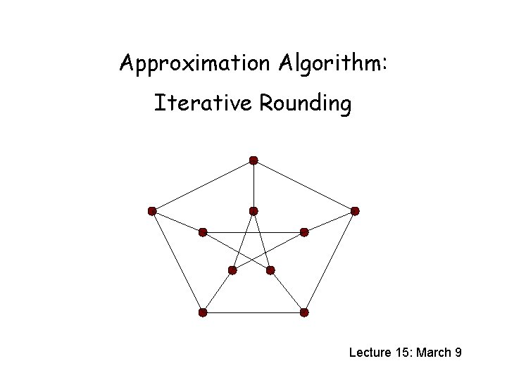
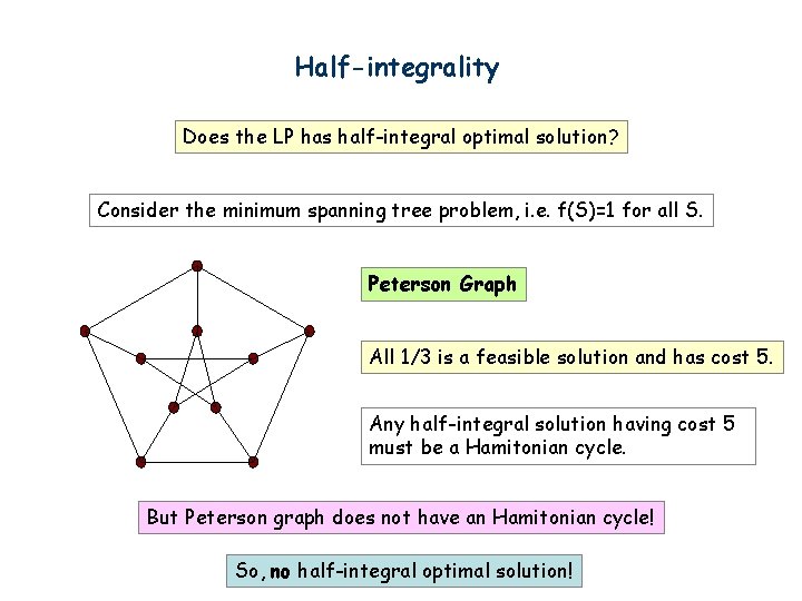
Half-integrality Does the LP has half-integral optimal solution? Consider the minimum spanning tree problem, i. e. f(S)=1 for all S. Peterson Graph All 1/3 is a feasible solution and has cost 5. Any half-integral solution having cost 5 must be a Hamitonian cycle. But Peterson graph does not have an Hamitonian cycle! So, no half-integral optimal solution!

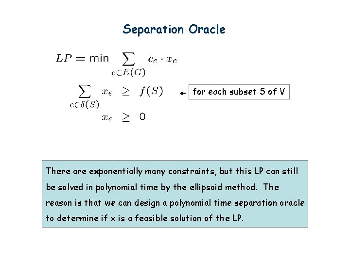
Separation Oracle for each subset S of V There are exponentially many constraints, but this LP can still be solved in polynomial time by the ellipsoid method. The reason is that we can design a polynomial time separation oracle to determine if x is a feasible solution of the LP.

Separation Oracle for each subset S of V Remember: f(S) = max{ r(u, v) | S separates u and v}. At least r(u, v) edges crossing S S u v Max-Flow Min-Cut Every (u, v)-cut has at least r(u, v) edges if and only if there are r(u, v) flows from u to v. Separation oracle: check if each pair u, v has a flow of r(u, v)!

Linear Programming Relaxation for each subset S of V What is the integrality gap of this LP?

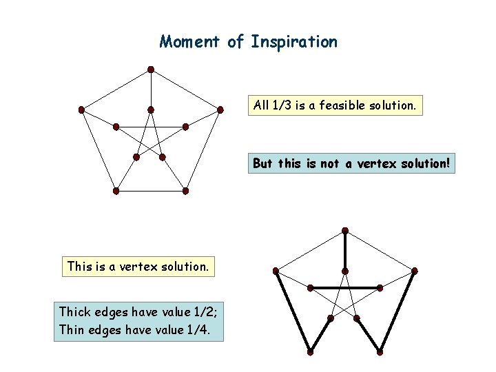
Moment of Inspiration All 1/3 is a feasible solution. But this is not a vertex solution! This is a vertex solution. Thick edges have value 1/2; Thin edges have value 1/4.

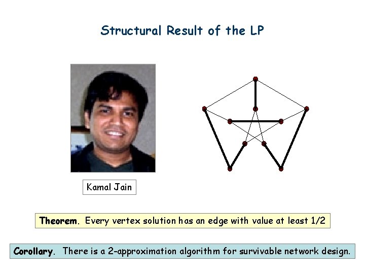
Structural Result of the LP Kamal Jain Theorem. Every vertex solution has an edge with value at least 1/2 Corollary. There is a 2 -approximation algorithm for survivable network design.

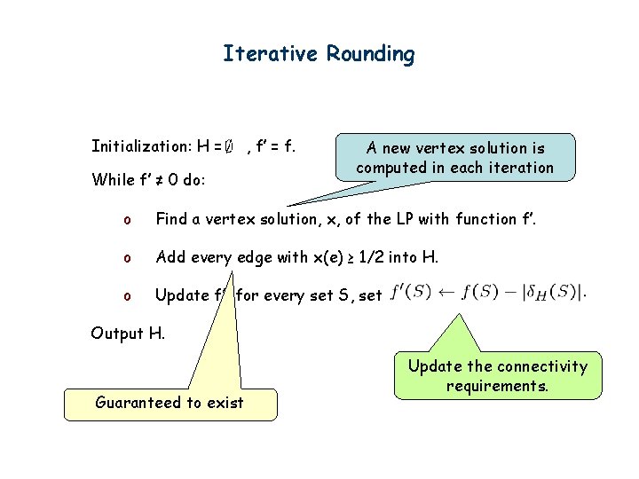
Iterative Rounding Initialization: H = While f’ ≠ 0 do: , f’ = f. A new vertex solution is computed in each iteration o Find a vertex solution, x, of the LP with function f’. o Add every edge with x(e) ≥ 1/2 into H. o Update f’: for every set S, set Output H. Guaranteed to exist Update the connectivity requirements.

Analysis Corollary. There is a 2 -approximation algorithm for survivable network design. Intuitive reason: we only pick an edge when the LP picks at least half. Proof: Let say we pick an edge e. Key: LP-c(e)x(e) is a feasible solution for the next iteration. cost(H) = c(e) + cost(H’) ≤ 2·c(e)x(e) + 2(LP-c(e)x(e)) ≤ 2 LP ≤ 2 OPT.

Some Remarks 1. The iterative rounding algorithm performs very well in practice. 2. No combinatorial algorithm has an performance ratio better than O(log n).

Spanning Tree with Degree Constraints Input • An undirected graph G = (V, E), • A degree upper bound k. Output • A spanning tree with degree at most k. NP-complete (Hamiltonian path when k=2).

Spanning Tree with Degree Constraints Motivation: to find a spanning tree in which there is no “overloaded” vertices. [Furer and Raghavachari ’ 92] Given k, there is a polynomial time algorithm which does the following: Either the algorithm (i) Show that there is no spanning tree with maximum degree at most k. (ii) Find a spanning tree with maximum degree at most k+1. In other words, there is an +1 algorithm for this problem!

Minimum Spanning Tree with Degree Constraints Input • An undirected graph G = (V, E), • A cost c(e) on each edge e, • A degree upper bound k. Output • A minimum spanning tree with degree at most k. Question: Is there a +1 algorithm for this problem as well? That is, a polytime algorithm which returns a minimum spanning tree with maximum degree at most k+1.

Conjecture Let OPT be the minimum cost of a spanning tree with maximum degree k. [Goemans] Conjecture: Given k, there is a polynomial time algorithm which returns a spanning tree with cost at most OPT and maximum degree at most k+1. Note that we do not restrict ourselves to MST.

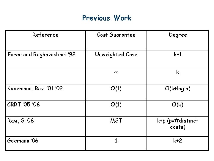
Previous Work Reference Cost Guarantee Degree Unweighted Case k+1 ∞ k Konemann, Ravi ’ 01 ’ 02 O(1) O(k+log n) CRRT ’ 05 ’ 06 O(1) O(k) Ravi, S. 06 MST k+p (p=#distinct costs) 1 k+2 Furer and Raghavachari ‘ 92 Goemans ’ 06

Our Result [Singh Lau 07] Theorem: Given k, there is a polynomial time algorithm which returns a spanning tree with cost at most OPT and maximum degree at most k+1. Technique: Adaptation of iterative rounding, but we do not round. Mohit Singh

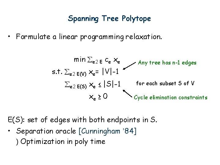
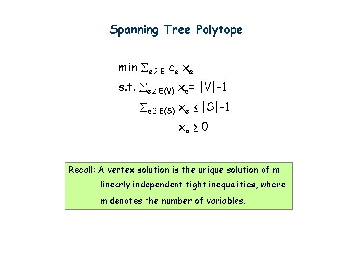
Spanning Tree Polytope • Formulate a linear programming relaxation. min e 2 E ce xe Any tree has n-1 edges s. t. e 2 E(V) xe= |V|-1 e 2 E(S) xe ≤ |S|-1 xe ≥ 0 for each subset S of V Cycle elimination constraints E(S): set of edges with both endpoints in S. • Separation oracle [Cunningham ’ 84] ) Optimization in poly time

Spanning Tree Polytope min e 2 E ce xe s. t. e 2 E(V) xe= |V|-1 e 2 E(S) xe ≤ |S|-1 xe ≥ 0 Recall: A vertex solution is the unique solution of m linearly independent tight inequalities, where m denotes the number of variables.

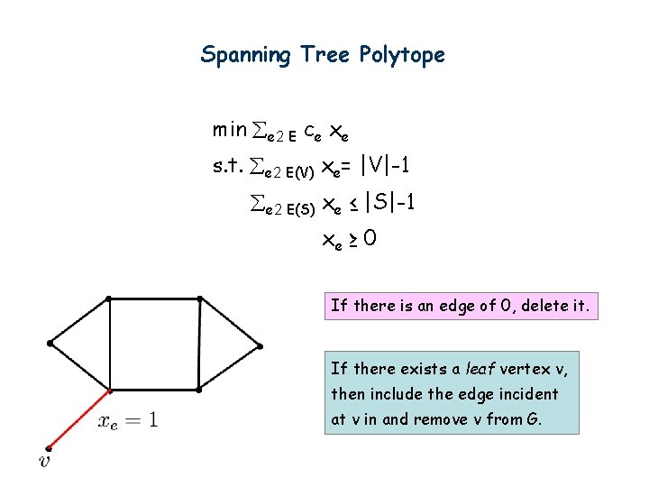
Spanning Tree Polytope min e 2 E ce xe s. t. e 2 E(V) xe= |V|-1 e 2 E(S) xe ≤ |S|-1 xe ≥ 0 If there is an edge of 0, delete it. If there exists a leaf vertex v, then include the edge incident at v in and remove v from G.

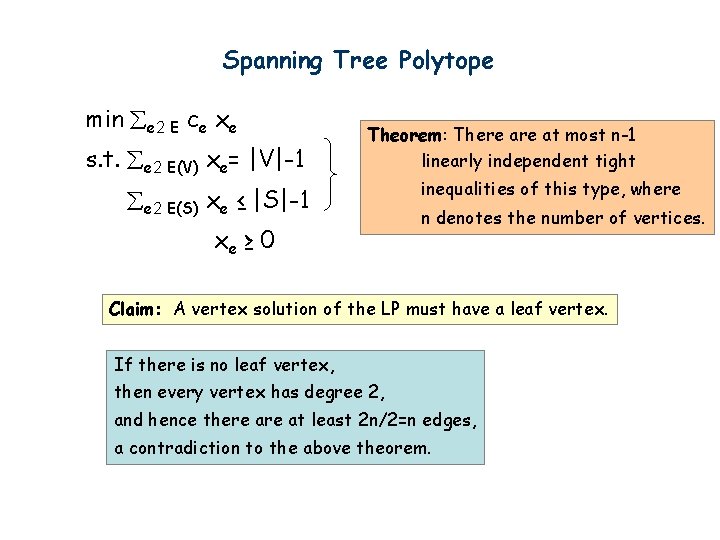
Spanning Tree Polytope min e 2 E ce xe s. t. e 2 E(V) xe= |V|-1 Theorem: There at most n-1 linearly independent tight e 2 E(S) xe ≤ |S|-1 xe ≥ 0 inequalities of this type, where n denotes the number of vertices. Claim: A vertex solution of the LP must have a leaf vertex. If there is no leaf vertex, then every vertex has degree 2, and hence there at least 2 n/2=n edges, a contradiction to the above theorem.

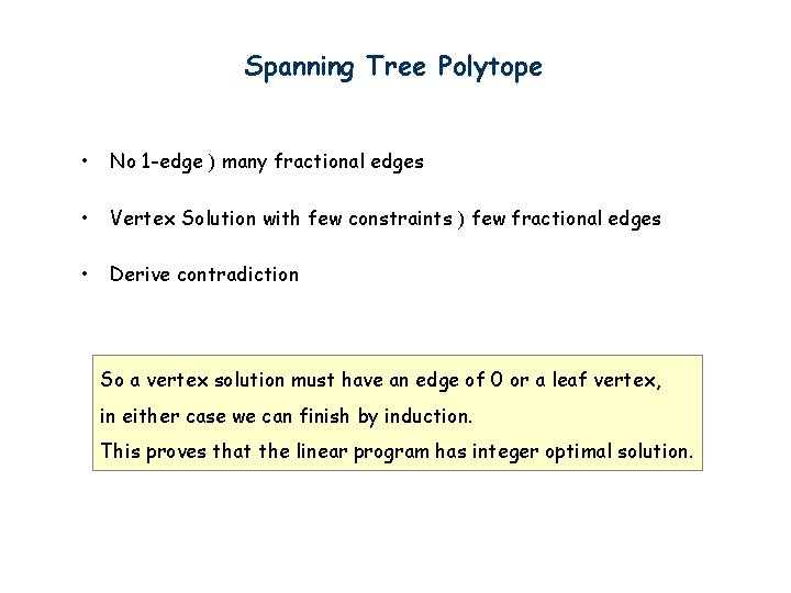
Spanning Tree Polytope • No 1 -edge ) many fractional edges • Vertex Solution with few constraints ) few fractional edges • Derive contradiction So a vertex solution must have an edge of 0 or a leaf vertex, in either case we can finish by induction. This proves that the linear program has integer optimal solution.

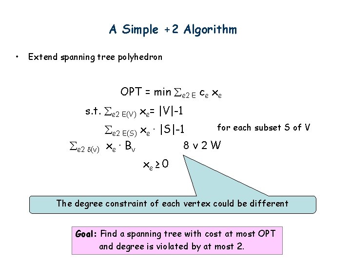
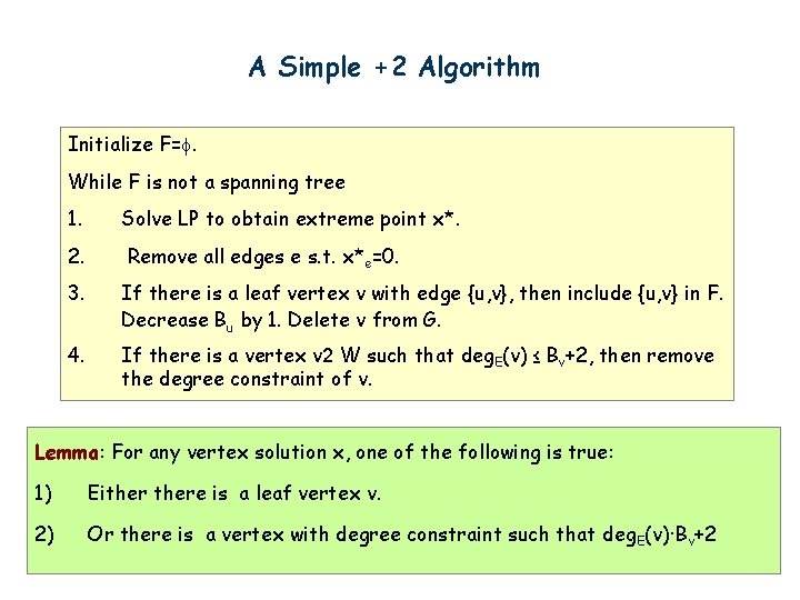
A Simple +2 Algorithm • Extend spanning tree polyhedron OPT = min e 2 E ce xe s. t. e 2 E(V) xe= |V|-1 e 2 (v) for each subset S of V e 2 E(S) xe · |S|-1 xe · B v 8 v 2 W xe ≥ 0 The degree constraint of each vertex could be different Goal: Find a spanning tree with cost at most OPT and degree is violated by at most 2.

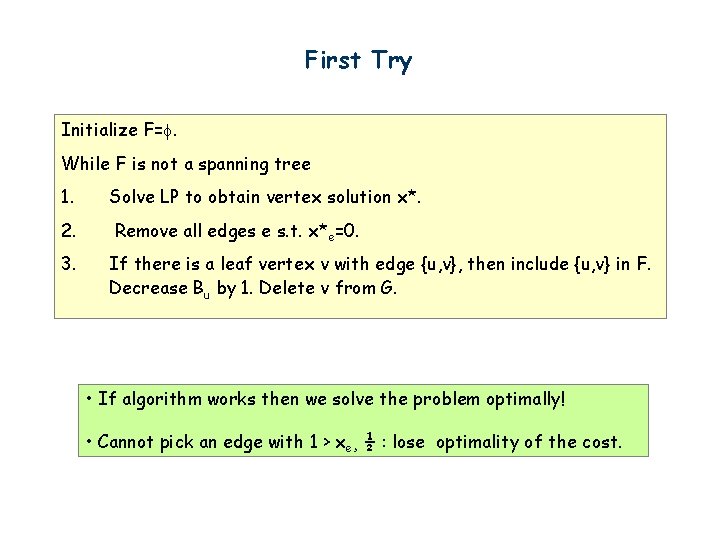
First Try Initialize F=. While F is not a spanning tree 1. Solve LP to obtain vertex solution x*. 2. Remove all edges e s. t. x*e=0. 3. If there is a leaf vertex v with edge {u, v}, then include {u, v} in F. Decrease Bu by 1. Delete v from G. • If algorithm works then we solve the problem optimally! • Cannot pick an edge with 1 > xe¸ ½ : lose optimality of the cost.

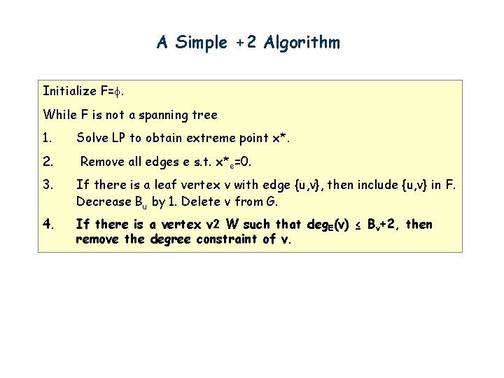
A Simple +2 Algorithm Initialize F=. While F is not a spanning tree 1. Solve LP to obtain extreme point x*. 2. Remove all edges e s. t. x*e=0. 3. If there is a leaf vertex v with edge {u, v}, then include {u, v} in F. Decrease Bu by 1. Delete v from G. 4. If there is a vertex v 2 W such that deg. E(v) ≤ Bv+2, then remove the degree constraint of v.

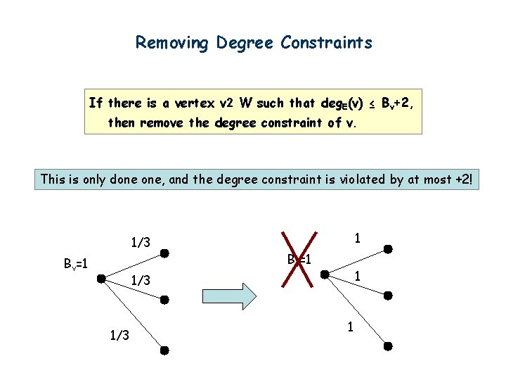
Removing Degree Constraints If there is a vertex v 2 W such that deg. E(v) ≤ Bv+2, then remove the degree constraint of v. This is only done one, and the degree constraint is violated by at most +2! 1/3 Bv=1 1 1/3 1

A Simple +2 Algorithm Initialize F=. While F is not a spanning tree 1. Solve LP to obtain extreme point x*. 2. Remove all edges e s. t. x*e=0. 3. If there is a leaf vertex v with edge {u, v}, then include {u, v} in F. Decrease Bu by 1. Delete v from G. 4. If there is a vertex v 2 W such that deg. E(v) ≤ Bv+2, then remove the degree constraint of v. Lemma: For any vertex solution x, one of the following is true: 1) Eithere is a leaf vertex v. 2) Or there is a vertex with degree constraint such that deg E(v)·Bv+2

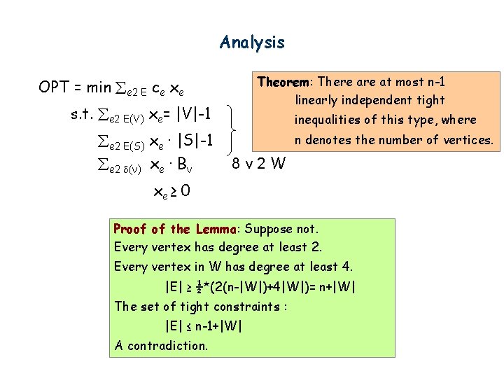
Analysis Theorem: There at most n-1 linearly independent tight OPT = min e 2 E ce xe s. t. e 2 E(V) xe= |V|-1 e 2 E(S) xe · |S|-1 e 2 (v) xe · Bv inequalities of this type, where n denotes the number of vertices. 8 v 2 W xe ≥ 0 Proof of the Lemma: Suppose not. Every vertex has degree at least 2. Every vertex in W has degree at least 4. |E| ≥ ½*(2(n-|W|)+4|W|)= n+|W| The set of tight constraints : |E| ≤ n-1+|W| A contradiction.

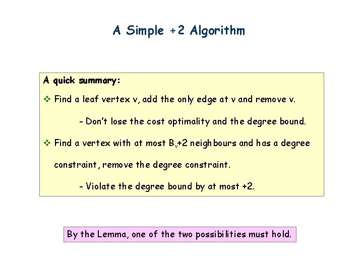
A Simple +2 Algorithm A quick summary: v Find a leaf vertex v, add the only edge at v and remove v. - Don’t lose the cost optimality and the degree bound. v Find a vertex with at most Bv+2 neighbours and has a degree constraint, remove the degree constraint. - Violate the degree bound by at most +2. By the Lemma, one of the two possibilities must hold.

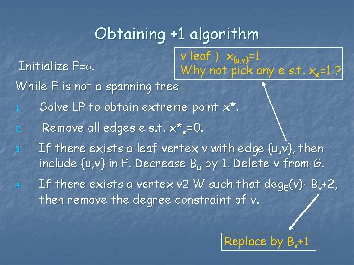
Obtaining +1 algorithm Initialize F=. While F is not a spanning tree 1. 2. 3. 4. v leaf ) x{u, v}=1 Why not pick any e s. t. xe=1 ? Solve LP to obtain extreme point x*. Remove all edges e s. t. x*e=0. If there exists a leaf vertex v with edge {u, v}, then include {u, v} in F. Decrease Bu by 1. Delete v from G. If there exists a vertex v 2 W such that deg. E(v)· Bv+2, then remove the degree constraint of v. Replace by Bv+1

Concluding Remarks 1. No combinatorial algorithm has a good performance ratio. 2. Similar techniques can be used for more general problems, e. g. minimum maximum degree k-ec subgraph 3. Can deal with lower and upper bounds. 4. A unifying framework for network design problems. 5. Proofs are based on uncrossing techniques in combinatorial optimiation.