Approximating functions polynomial interpolation Lagrange and Newtons divided

Approximating functions, polynomial interpolation (Lagrange and Newton’s divided differences) formulas, error approximations 1

Introduction to Interpolation p. Introduction p. Interpolation Problem p. Existence and Uniqueness p. Linear and Quadratic Interpolation p. Newton’s Divided Difference Method p. Properties of Divided Differences 2

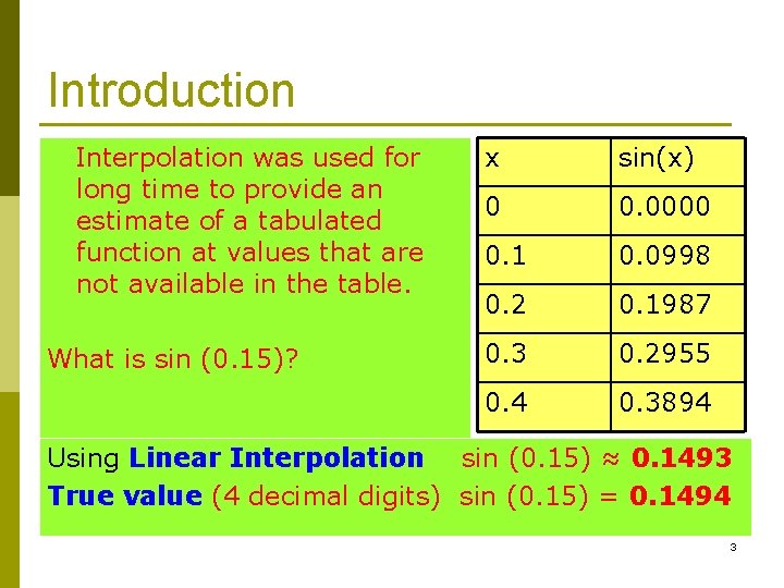
Introduction Interpolation was used for long time to provide an estimate of a tabulated function at values that are not available in the table. What is sin (0. 15)? x sin(x) 0 0. 0000 0. 1 0. 0998 0. 2 0. 1987 0. 3 0. 2955 0. 4 0. 3894 Using Linear Interpolation sin (0. 15) ≈ 0. 1493 True value (4 decimal digits) sin (0. 15) = 0. 1494 3

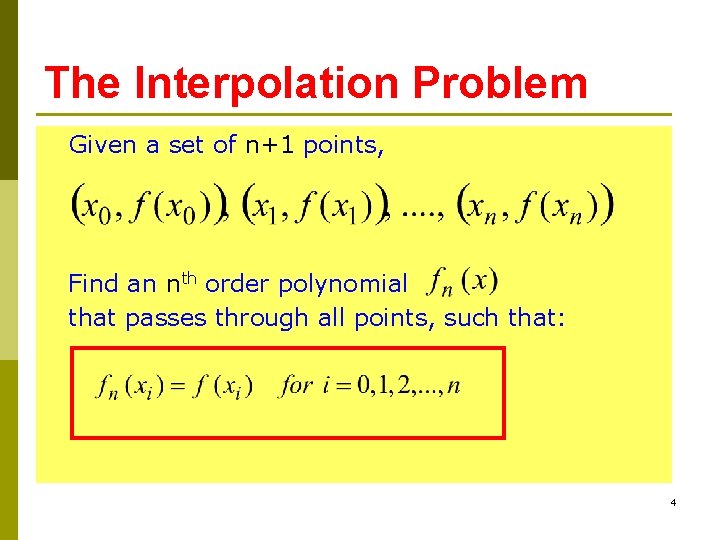
The Interpolation Problem Given a set of n+1 points, Find an nth order polynomial that passes through all points, such that: 4

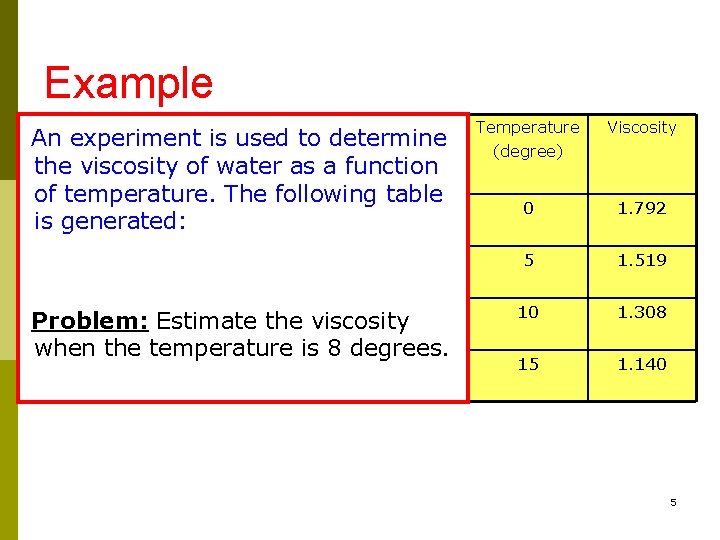
Example An experiment is used to determine the viscosity of water as a function of temperature. The following table is generated: Problem: Estimate the viscosity when the temperature is 8 degrees. Temperature (degree) Viscosity 0 1. 792 5 1. 519 10 1. 308 15 1. 140 5

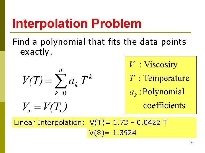
Interpolation Problem Find a polynomial that fits the data points exactly. Linear Interpolation: V(T)= 1. 73 − 0. 0422 T V(8)= 1. 3924 6

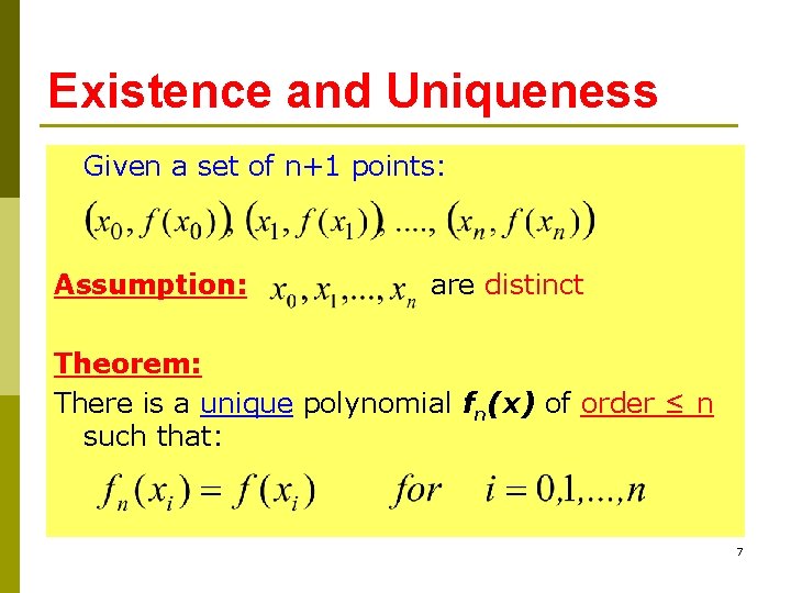
Existence and Uniqueness Given a set of n+1 points: Assumption: are distinct Theorem: There is a unique polynomial fn(x) of order ≤ n such that: 7

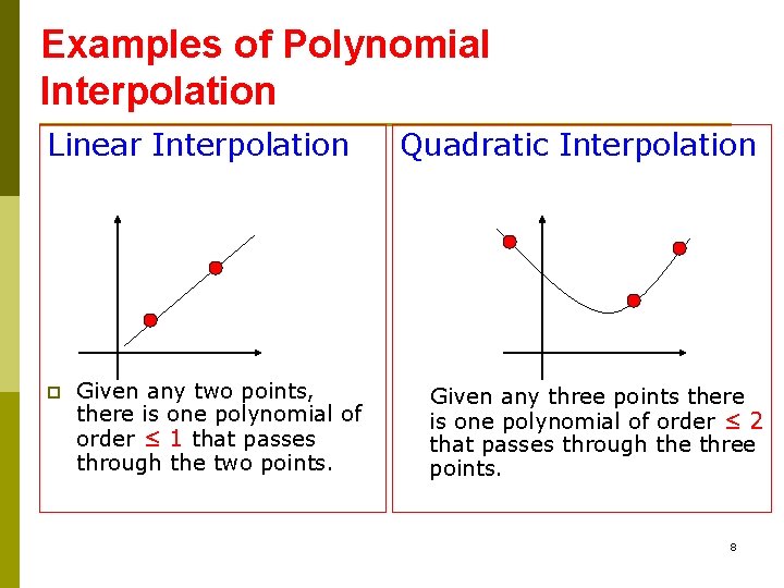
Examples of Polynomial Interpolation Linear Interpolation p Given any two points, there is one polynomial of order ≤ 1 that passes through the two points. Quadratic Interpolation Given any three points there is one polynomial of order ≤ 2 that passes through the three points. 8

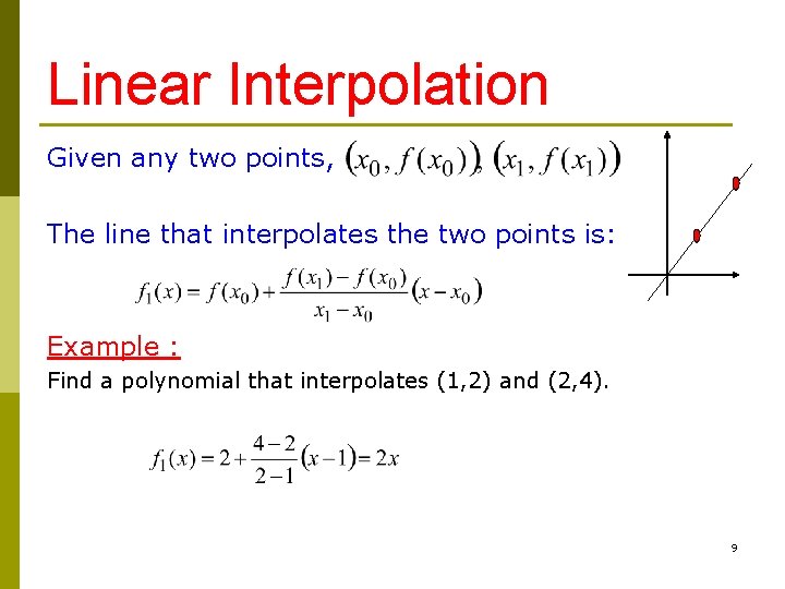
Linear Interpolation Given any two points, The line that interpolates the two points is: Example : Find a polynomial that interpolates (1, 2) and (2, 4). 9

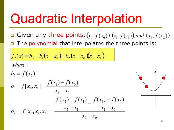
Quadratic Interpolation p Given any three points: p The polynomial that interpolates the three points is: 10

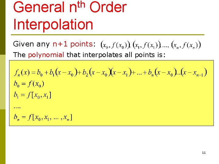
General nth Order Interpolation Given any n+1 points: The polynomial that interpolates all points is: 11

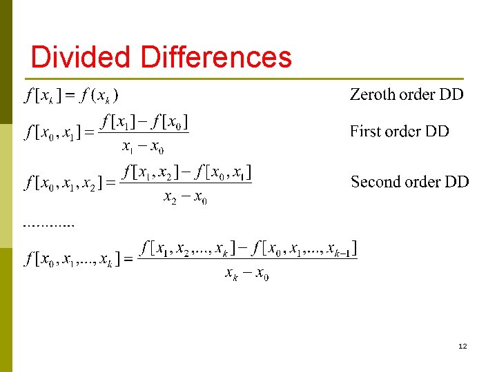
Divided Differences 12

Divided Difference Table x F[ ] F[ , , , ] x 0 F[x 0] F[x 0, x 1, x 2] F[x 0, x 1, x 2, x 3] x 1 F[x 1] F[x 1, x 2, x 3] x 2 F[x 2] F[x 2, x 3] x 3 F[x 3] 13

Divided Difference Table x F[ ] F[ , , ] 0 -5 2 -4 1 -3 6 -1 -15 Entries of the divided difference table are obtained from the data table using simple operations. f(xi) 0 -5 1 -3 -1 -15 14

Divided Difference Table x F[ ] F[ , , ] 0 -5 2 -4 1 -3 6 -1 -15 f(xi) 0 1 -1 -5 -3 -15 The first two column of the table are the data columns. Third column: First order differences. Fourth column: Second order differences. 15

Divided Difference Table x F[ ] F[ , , ] 0 -5 2 -4 1 -3 6 -1 -15 0 -5 1 -3 -1 -15 16

Divided Difference Table x F[ ] F[ , , ] 0 -5 2 -4 1 -3 6 -1 -15 0 -5 1 -3 -1 -15 17

Divided Difference Table x F[ ] F[ , , ] 0 -5 2 -4 1 -3 6 -1 -15 0 -5 1 -3 -1 -15 18

Divided Difference Table x F[ ] F[ , , ] 0 -5 2 -4 1 -3 6 -1 -15 0 -5 1 -3 -1 -15 f 2(x)= F[x 0]+F[x 0, x 1] (x-x 0)+F[x 0, x 1, x 2] (x-x 0)(x-x 1) 19

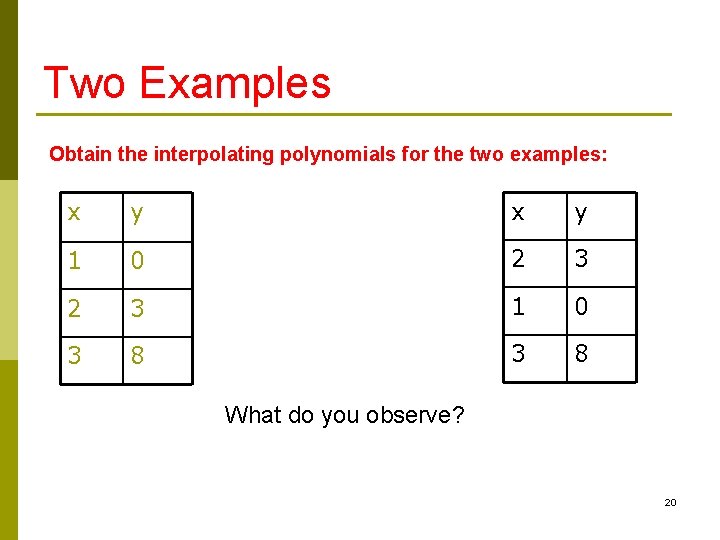
Two Examples Obtain the interpolating polynomials for the two examples: x y 1 0 2 3 1 0 3 8 What do you observe? 20

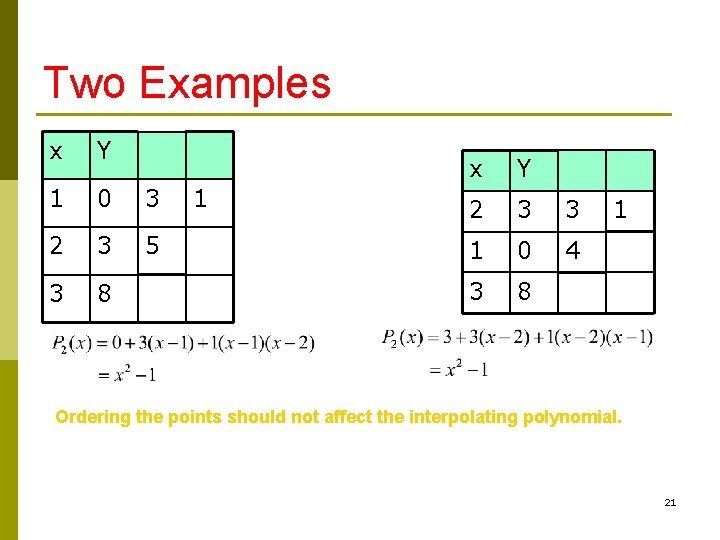
Two Examples x Y 1 0 3 2 3 5 3 8 1 x Y 2 3 3 1 0 4 3 8 1 Ordering the points should not affect the interpolating polynomial. 21

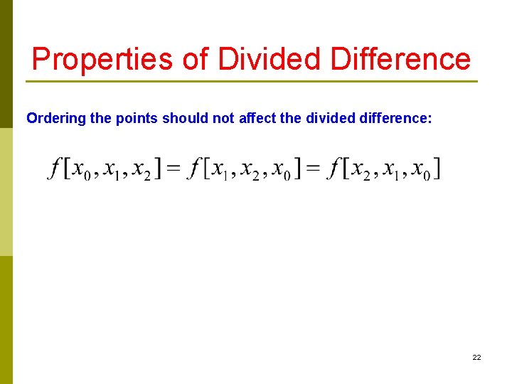
Properties of Divided Difference Ordering the points should not affect the divided difference: 22

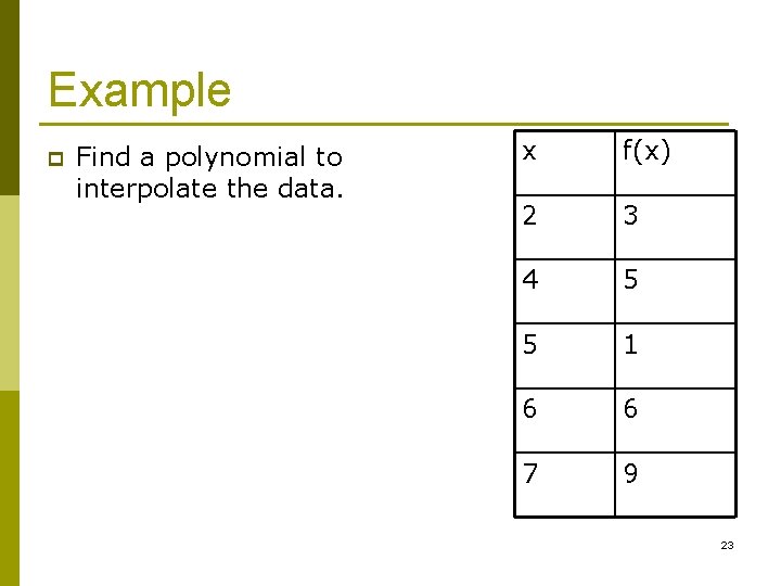
Example p Find a polynomial to interpolate the data. x f(x) 2 3 4 5 5 1 6 6 7 9 23

Example x 2 4 5 f(x) f[ , ] 3 1 5 -4 1 5 6 7 6 9 f[ , , ] -1. 6667 4. 5 -1 f[ , , , ] 1. 5417 -1. 8333 f[ , , ] -0. 6750 3 24

Summary 25

Lagrange Interpolation 26

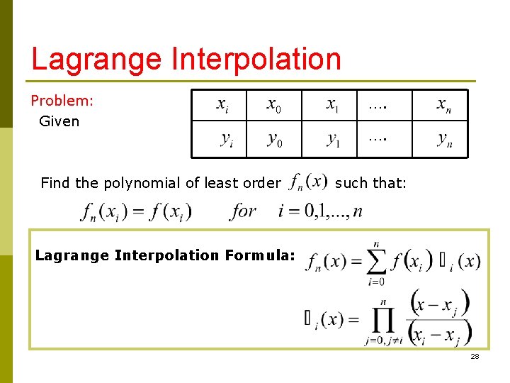
The Interpolation Problem Given a set of n+1 points: Find an nth order polynomial: that passes through all points, such that: 27

Lagrange Interpolation Problem: Given Find the polynomial of least order …. …. such that: Lagrange Interpolation Formula: 28

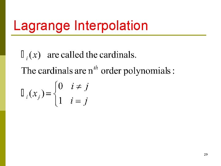
Lagrange Interpolation 29

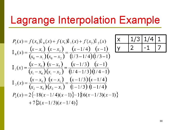
Lagrange Interpolation Example x y 1/3 1/4 1 2 -1 7 30

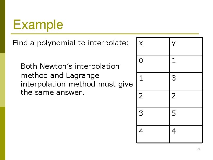
Example Find a polynomial to interpolate: x y 0 1 Both Newton’s interpolation method and Lagrange 1 interpolation method must give the same answer. 2 3 5 4 4 31

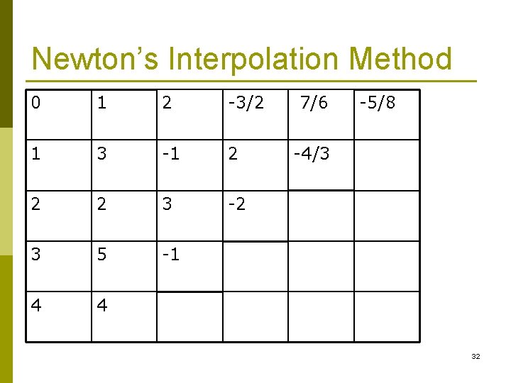
Newton’s Interpolation Method 0 1 2 -3/2 1 3 -1 2 2 2 3 -2 3 5 -1 4 4 7/6 -5/8 -4/3 32

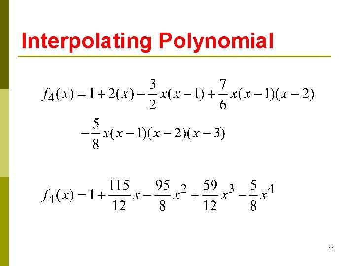
Interpolating Polynomial 33

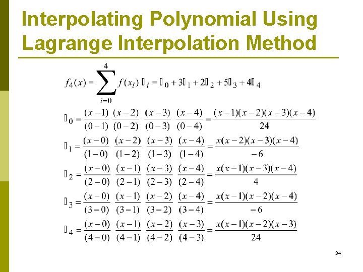
Interpolating Polynomial Using Lagrange Interpolation Method 34

Inverse Interpolation Error in Polynomial Interpolation 35

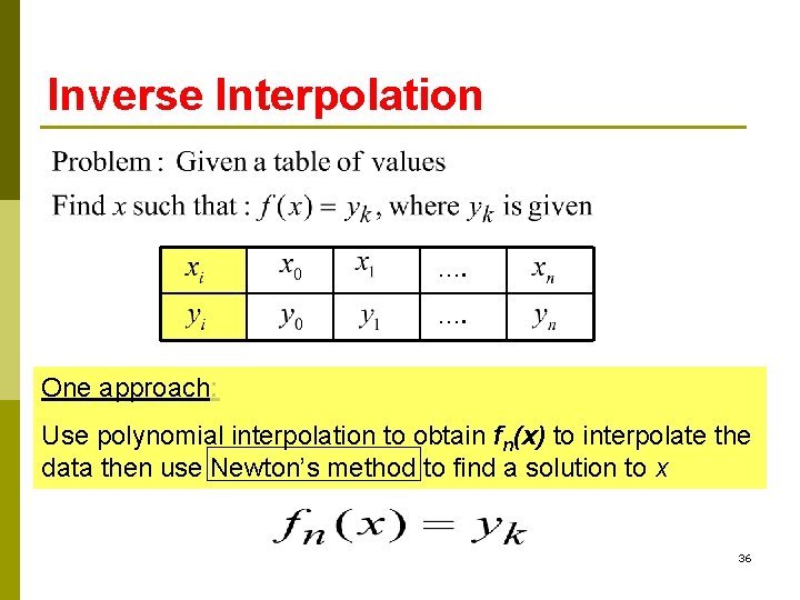
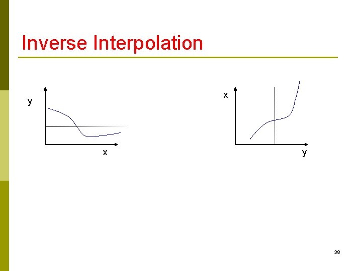
Inverse Interpolation …. …. One approach: Use polynomial interpolation to obtain fn(x) to interpolate the data then use Newton’s method to find a solution to x 36

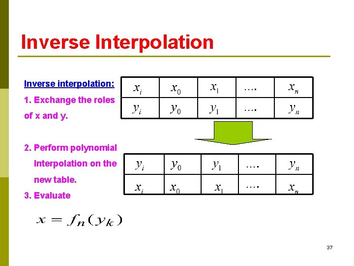
Inverse Interpolation Inverse interpolation: …. 1. Exchange the roles …. of x and y. 2. Perform polynomial Interpolation on the …. new table. …. 3. Evaluate 37

Inverse Interpolation x y 38

Inverse Interpolation Question: What is the limitation of inverse interpolation? • The original function has an inverse. • y 1, y 2, …, yn must be distinct. 39

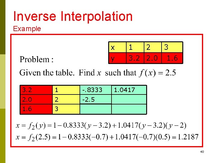
Inverse Interpolation Example x y 3. 2 1 -. 8333 2. 0 2 -2. 5 1. 6 3 1 2 3 3. 2 2. 0 1. 6 1. 0417 40

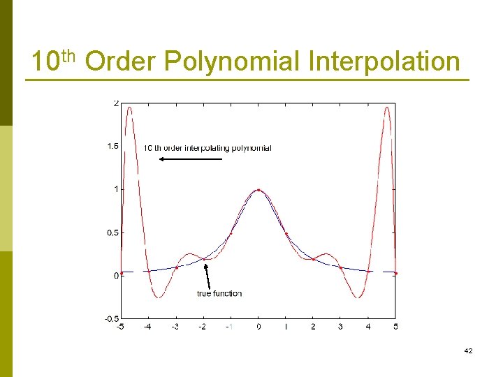
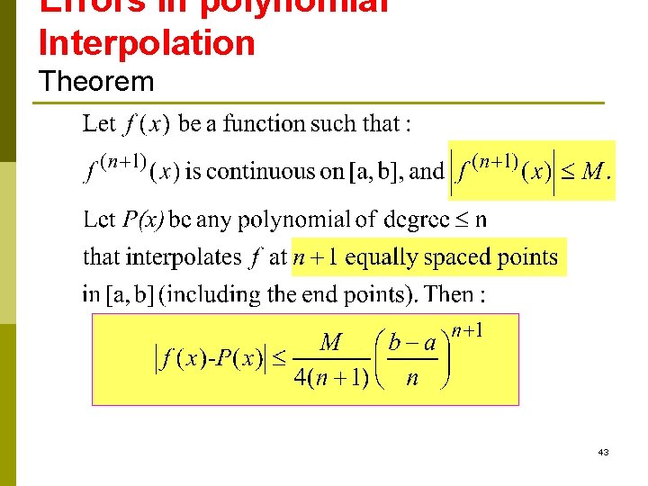
Errors in polynomial Interpolation p Polynomial interpolation may lead to large errors (especially for high order polynomials). BE CAREFUL p When an nth order interpolating polynomial is used, the error is related to the (n+1)th order derivative. 41

10 th Order Polynomial Interpolation 42

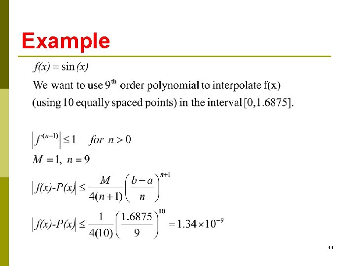
Errors in polynomial Interpolation Theorem 43

Example 44

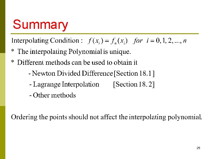
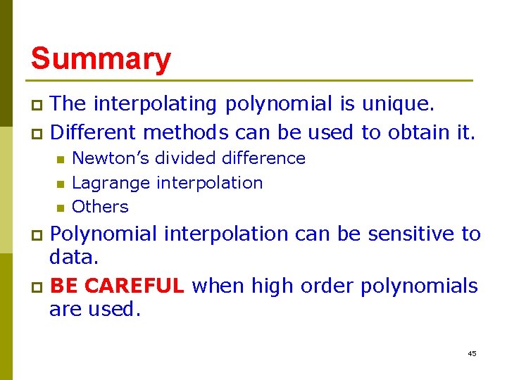
Summary The interpolating polynomial is unique. p Different methods can be used to obtain it. p n n n Newton’s divided difference Lagrange interpolation Others Polynomial interpolation can be sensitive to data. p BE CAREFUL when high order polynomials are used. p 45