Approximate methods for calculating probability of failure Monte

Approximate methods for calculating probability of failure • Monte Carlo simulation • First-order second-moment method (FOSM) • Working with normal distributions is appealing – The reliability index • Most probable point • First order reliability method (FORM) • The Rosenblatt transformation

SOURCE: http: //www. sz-wholesale. com/upload. Files/041022104413 s. jpg Monte Carlo Simulation • Given a random variable X and a function h(X): sample X: [x 1, x 2, …, xn]; Calculate [h(x 1), h(x 2), …, h(xn)]; use to approximate statistics of h. • Example: X is U[0, 1]. Use MCS to find mean of X 2 x=rand(10); y=x. ^2; %generates 10 x 10 random matrix sumy=sum(y)/10 sumy =0. 4017 0. 5279 0. 1367 0. 3501 0. 3072 0. 3362 0. 3855 0. 3646 0. 5033 0. 2666 sum(sumy)/10 ans =0. 3580 • What is the true mean SOURCE: http: //schools. sd 68. bc. ca/ed 611/akerley/question. jpg

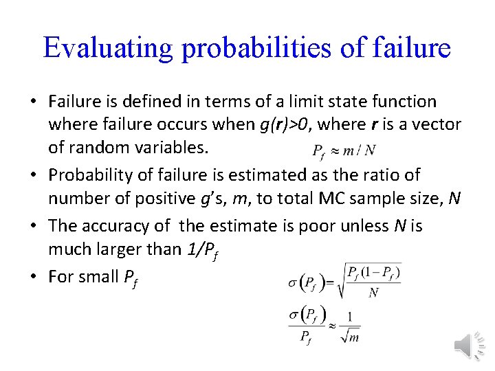
Evaluating probabilities of failure • Failure is defined in terms of a limit state function where failure occurs when g(r)>0, where r is a vector of random variables. • Probability of failure is estimated as the ratio of number of positive g’s, m, to total MC sample size, N • The accuracy of the estimate is poor unless N is much larger than 1/Pf • For small Pf

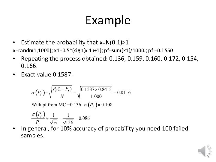
Example • Estimate the probability that x=N(0, 1)>1 x=randn(1, 1000); x 1=0. 5*(sign(x-1)+1); pf=sum(x 1)/1000. ; pf =0. 1550 • Repeating the process obtained: 0. 136, 0. 159, 0. 160, 0. 172, 0. 154, 0. 166. • Exact value 0. 1587. • In general, for 10% accuracy of probability you need 100 failed samples.

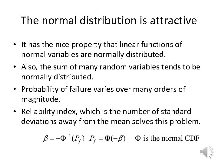
The normal distribution is attractive • It has the nice property that linear functions of normal variables are normally distributed. • Also, the sum of many random variables tends to be normally distributed. • Probability of failure varies over many orders of magnitude. • Reliability index, which is the number of standard deviations away from the mean solves this problem.

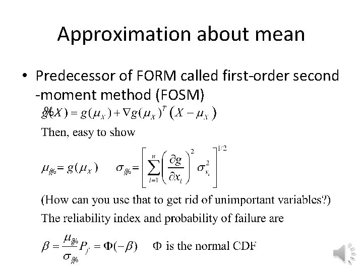
Approximation about mean • Predecessor of FORM called first-order second -moment method (FOSM)

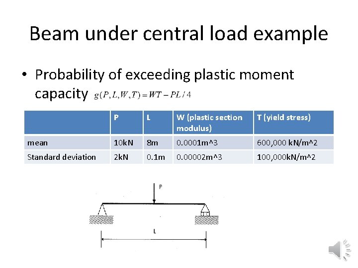
Beam under central load example • Probability of exceeding plastic moment capacity P L W (plastic section modulus) T (yield stress) mean 10 k. N 8 m 0. 0001 m^3 600, 000 k. N/m^2 Standard deviation 2 k. N 0. 1 m 0. 00002 m^3 100, 000 k. N/m^2

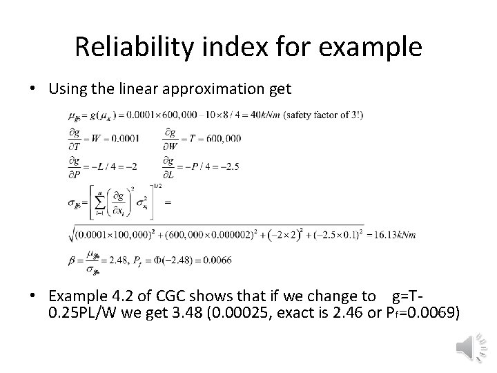
Reliability index for example • Using the linear approximation get • Example 4. 2 of CGC shows that if we change to g=T 0. 25 PL/W we get 3. 48 (0. 00025, exact is 2. 46 or Pf=0. 0069)

Most probable point (MPP) • The error due to the linear approximation is exacerbated due to the fact that the expansion may be about a point that is far from the failure region (due to the safety margin). • Hasofer and Lind suggested remedying this problem by finding the most probable point and linearizing about it. • The joint distribution of all the random variables assigns a probability density to every point in the random space. The point with the highest density on the line g=0 is the MPP.

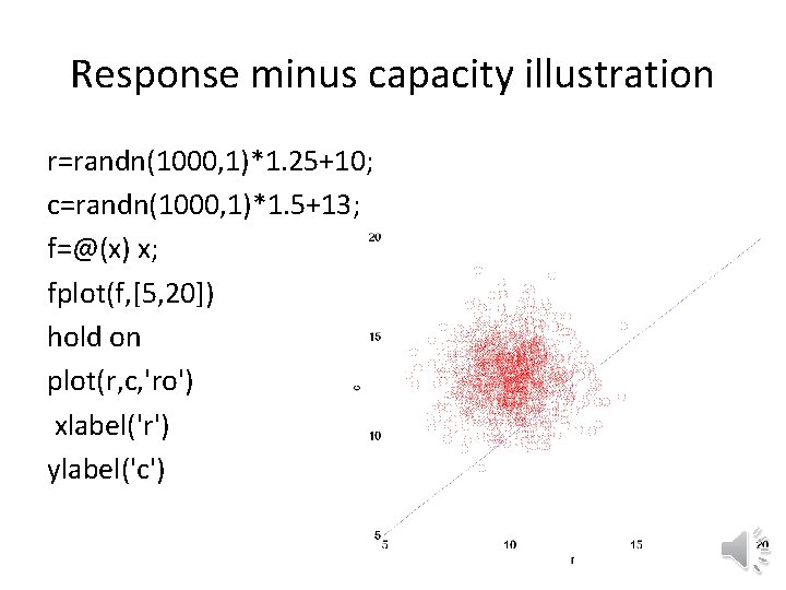
Response minus capacity illustration r=randn(1000, 1)*1. 25+10; c=randn(1000, 1)*1. 5+13; f=@(x) x; fplot(f, [5, 20]) hold on plot(r, c, 'ro') xlabel('r') ylabel('c')

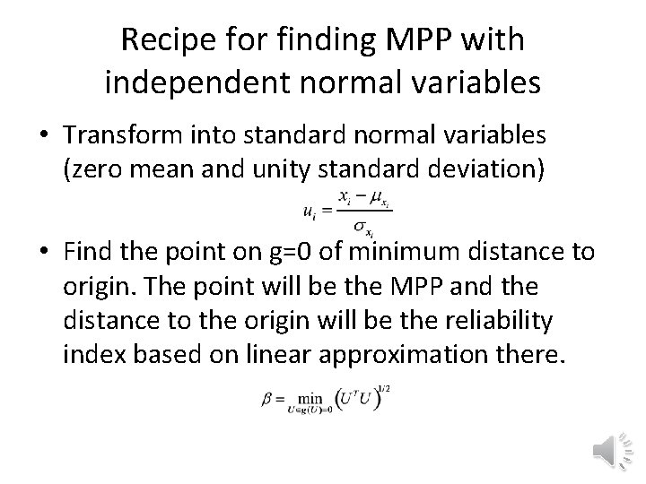
Recipe for finding MPP with independent normal variables • Transform into standard normal variables (zero mean and unity standard deviation) • Find the point on g=0 of minimum distance to origin. The point will be the MPP and the distance to the origin will be the reliability index based on linear approximation there.

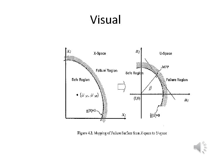
Visual

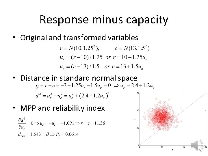
Response minus capacity • Original and transformed variables • Distance in standard normal space • MPP and reliability index

First order reliability method (FORM) • Limit state g(X). Failure when g<0. • Linear approximation of limit state together with assumption that random variables are normal. • Approximate around most probable point. • Then limit state is also normal variable. • Reliability index is the distance of the mean of g from zero measured in standard deviations.

General case • If random variables are normal but correlated, a linear transformation will transform them to independent variables. • If random variables are not normal, can be transformed to normal with similar probability of failure. See Section 4. 1. 5 of CGC (It is called the Rosenblatt transformation) • Murray Rosenblatt, Remarks on a Multivariate Transformation, Ann. Math. Statist. Volume 23, Number 3 (1952), 470 -472.