Approximate Dynamic Programming in Rail Operations June 2007

Approximate Dynamic Programming in Rail Operations June, 2007 Tristan VI Phuket Island, Thailand Warren Powell Belgacem Bouzaiene-Ayari CASTLE Laboratory Princeton University http: //www. castlelab. princeton. edu © Warren B. Powell 2007 © 2000 Warren B. Powell, Princeton University

© Warren B. Powell 2007 2

© Warren B. Powell 2007

© Warren B. Powell 2007 4

© Warren B. Powell 2007

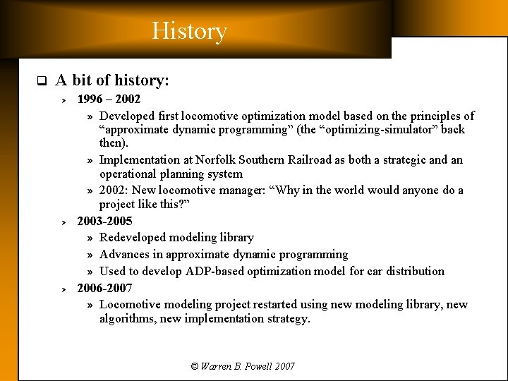
History q A bit of history: Ø Ø Ø 1996 – 2002 » Developed first locomotive optimization model based on the principles of “approximate dynamic programming” (the “optimizing-simulator” back then). » Implementation at Norfolk Southern Railroad as both a strategic and an operational planning system » 2002: New locomotive manager: “Why in the world would anyone do a project like this? ” 2003 -2005 » Redeveloped modeling library » Advances in approximate dynamic programming » Used to develop ADP-based optimization model for car distribution 2006 -2007 » Locomotive modeling project restarted using new modeling library, new algorithms, new implementation strategy. © Warren B. Powell 2007

Outline q q q The locomotive planning problem Approximate dynamic programming Solving the subproblem Decomposition strategy Implementation © Warren B. Powell 2007

Outline q q q The locomotive planning problem Approximate dynamic programming Solving the subproblem Decomposition strategy Implementation © Warren B. Powell 2007

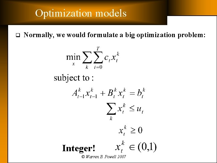
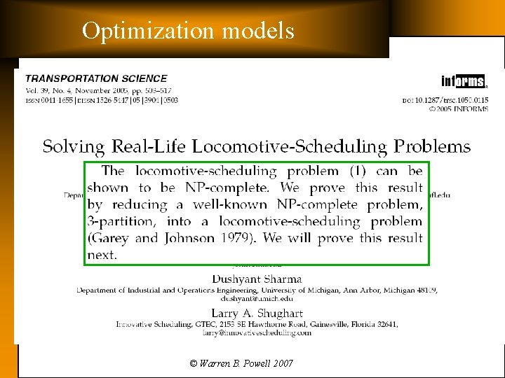
Optimization models q Normally, we would formulate a big optimization problem: Integer! © Warren B. Powell 2007

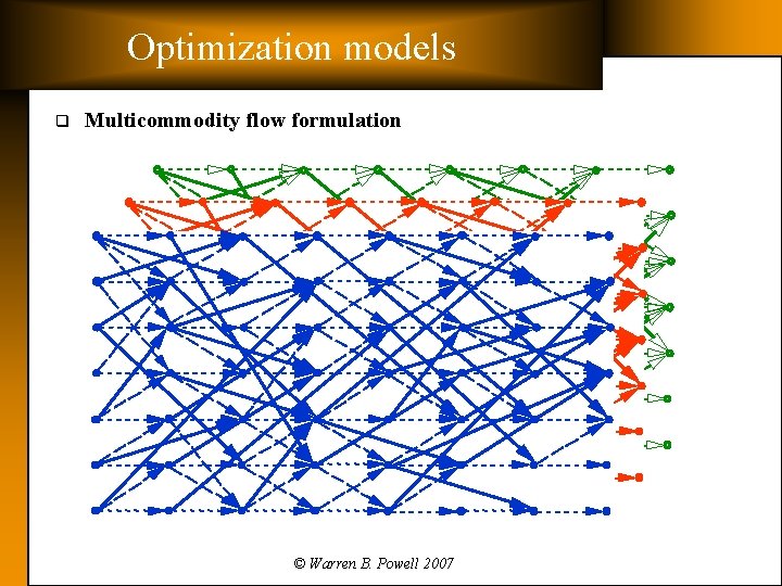
Optimization models q Multicommodity flow formulation © Warren B. Powell 2007

Optimization models q Multicommodity flow formulation © Warren B. Powell 2007

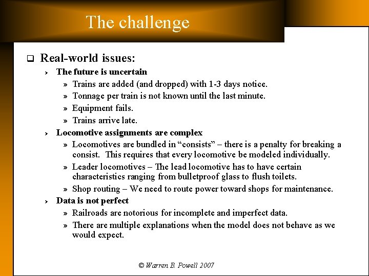
The challenge q Real-world issues: Ø Ø Ø The future is uncertain » Trains are added (and dropped) with 1 -3 days notice. » Tonnage per train is not known until the last minute. » Equipment fails. » Trains arrive late. Locomotive assignments are complex » Locomotives are bundled in “consists” – there is a penalty for breaking a consist. This requires that every locomotive be modeled individually. » Leader locomotives – The lead locomotive has to have certain characteristics ranging from bulletproof glass to flush toilets. » Shop routing – We need to route power toward shops for maintenance. Data is not perfect » Railroads are notorious for incomplete and imperfect data. » There are multiple explanations when the model does not behave as we would expect. © Warren B. Powell 2007

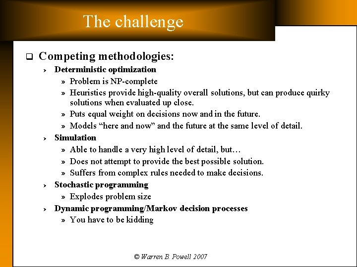
The challenge q Competing methodologies: Ø Ø Deterministic optimization » Problem is NP-complete » Heuristics provide high-quality overall solutions, but can produce quirky solutions when evaluated up close. » Puts equal weight on decisions now and in the future. » Models “here and now” and the future at the same level of detail. Simulation » Able to handle a very high level of detail, but… » Does not attempt to provide the best possible solution. » Suffers from complex rules needed to make decisions. Stochastic programming » Explodes problem size Dynamic programming/Markov decision processes » You have to be kidding © Warren B. Powell 2007

Outline q q q The locomotive planning problem Approximate dynamic programming Solving the subproblem Decomposition strategy Implementation © Warren B. Powell 2007

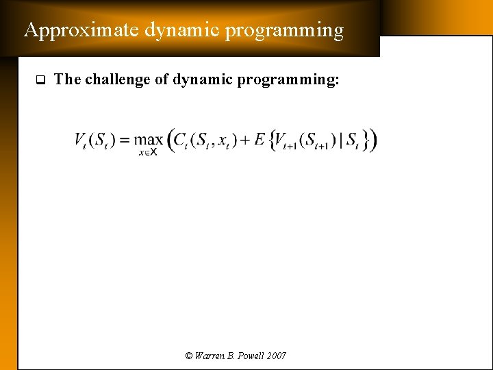
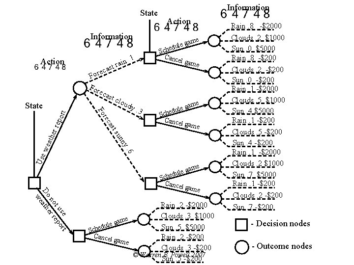
Approximate dynamic programming q The challenge of dynamic programming: Three curses q Problem: Curse of dimensionality State space Outcome space Action space (feasible region) © Warren B. Powell 2007

State Information Action ain st r eca r o F For eca rt epo er r y. 3 Action e gam e l u d Sche Cance l gam e ame g e l edu Sch Cancel game ny n su. 6 wea th oud ast rec Use st c l Fo State . 1 Information se rt t u po no er re Do ath we e gam e l u d Sche Cancel game Rain. 2 -$2000 Clouds. 3 $1000 me a g dule Sun. 5 $5000 Sche Cancel Rain. 2 -$200 game Clouds. 3 -$200 © Warren B. Powell 2007 Sun. 5 -$200 Rain. 8 -$2000 Clouds. 2 $1000 Sun. 0 $5000 Rain. 8 -$200 Clouds. 2 -$200 Sun. 0 -$200 Rain. 1 -$2000 Clouds. 5 $1000 Sun. 4 $5000 Rain. 1 -$200 Clouds. 5 -$200 Sun. 4 -$200 Rain. 1 -$2000 Clouds. 2 $1000 Sun. 7 $5000 Rain. 1 -$200 Clouds. 2 -$200 Sun. 7 -$200 - Decision nodes - Outcome nodes

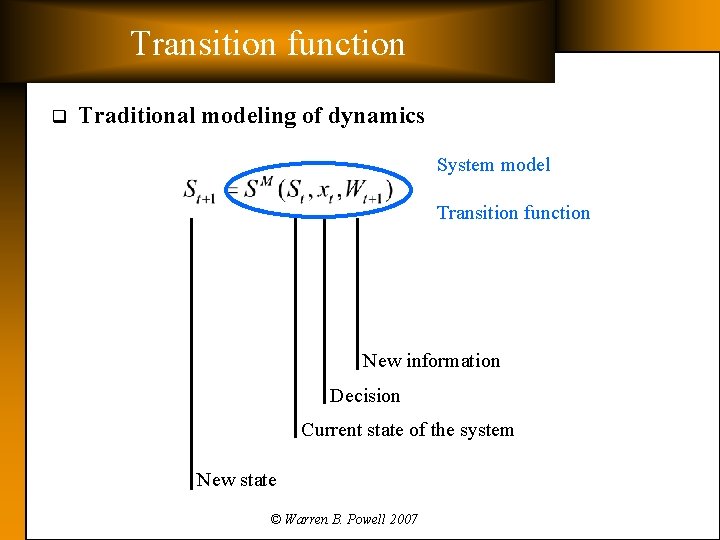
Transition function q Traditional modeling of dynamics System model Transition function New information Decision Current state of the system New state © Warren B. Powell 2007

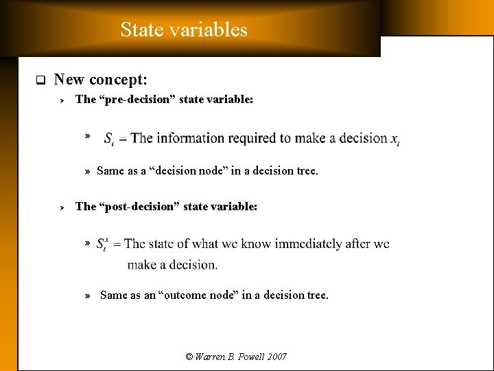
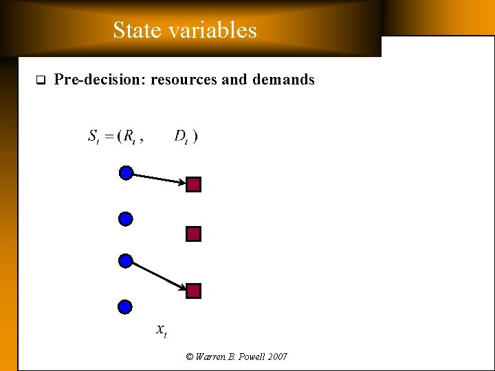
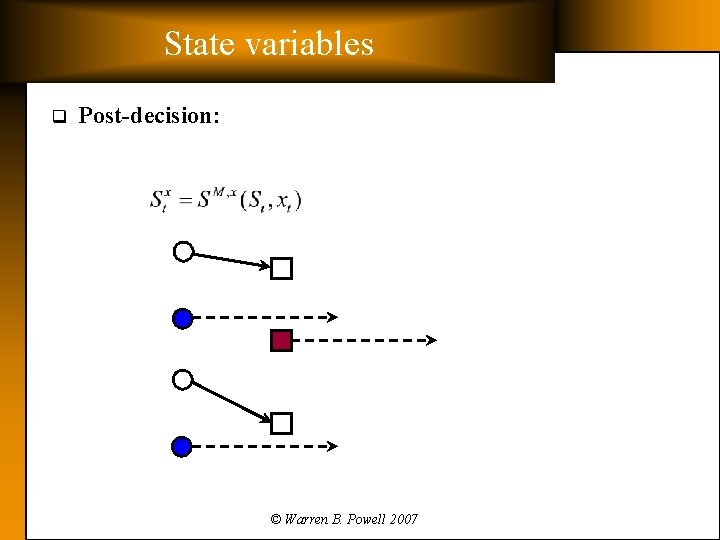
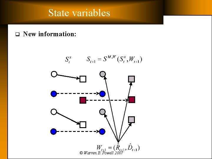
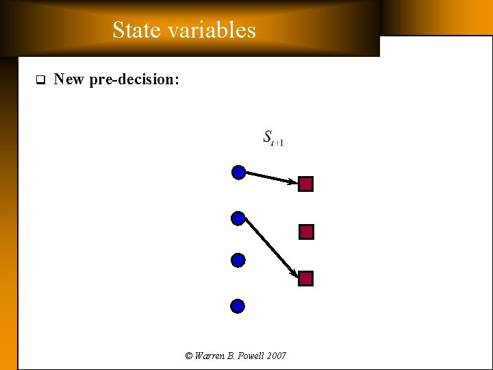
State variables q New concept: Ø The “pre-decision” state variable: » » Same as a “decision node” in a decision tree. Ø The “post-decision” state variable: » » Same as an “outcome node” in a decision tree. © Warren B. Powell 2007

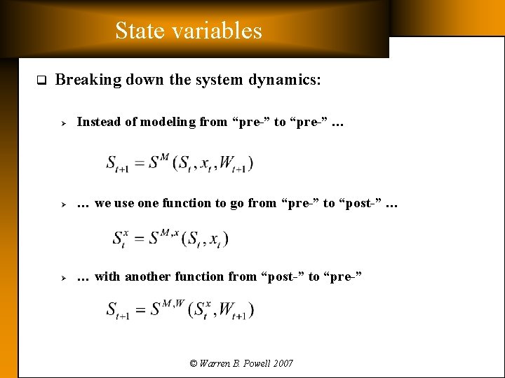
State variables q Breaking down the system dynamics: Ø Instead of modeling from “pre-” to “pre-” … Ø … we use one function to go from “pre-” to “post-” … Ø … with another function from “post-” to “pre-” © Warren B. Powell 2007

State variables q Pre-decision: resources and demands © Warren B. Powell 2007

State variables q Post-decision: © Warren B. Powell 2007

State variables q New information: © Warren B. Powell 2007

State variables q New pre-decision: © Warren B. Powell 2007

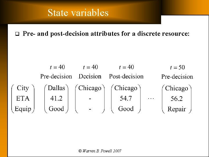
State variables q Pre- and post-decision attributes for a discrete resource: … © Warren B. Powell 2007

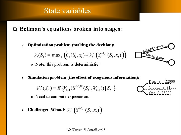
State variables q Bellman’s equations broken into stages: Ø Optimization problem (making the decision): me e ga edul Sch Cance l gam e » Note: this problem is deterministic! Ø Simulation problem (the effect of exogenous information): » Need to compute expectation. Ø Challenge: What is © Warren B. Powell 2007 Rain. 8 -$2000 Clouds. 2 $1000 Sun. 0 $5000

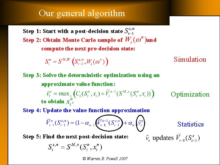
Our general algorithm Step 1: Start with a post-decision state Step 2: Obtain Monte Carlo sample of compute the next pre-decision state: and Simulation Step 3: Solve the deterministic optimization using an approximate value function: to obtain. Step 4: Update the value function approximation Optimization Statistics Step 5: Find the next post-decision state: © Warren B. Powell 2007

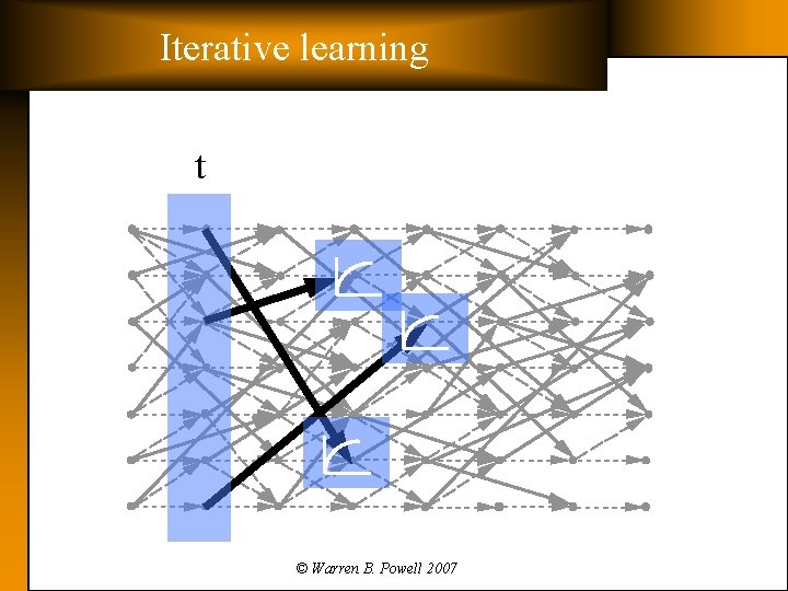
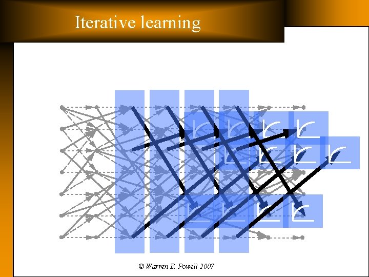
Iterative learning t © Warren B. Powell 2007

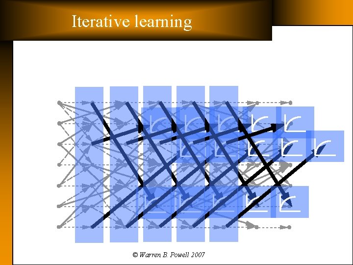
Iterative learning © Warren B. Powell 2007

Iterative learning © Warren B. Powell 2007

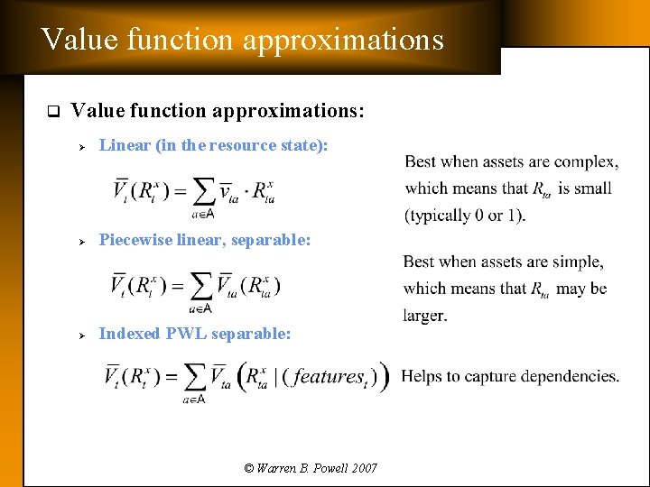
Value function approximations q Value function approximations: Ø Linear (in the resource state): Ø Piecewise linear, separable: Ø Indexed PWL separable: © Warren B. Powell 2007

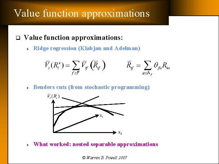
Value function approximations q Value function approximations: Ø Ridge regression (Klabjan and Adelman) Ø Benders cuts (from stochastic programming) Ø What worked: nested separable approximations © Warren B. Powell 2007

Coming in September, 2007 ? ? © Warren B. Powell 2007

Outline q q q The locomotive planning problem Approximate dynamic programming Solving the subproblem Decomposition strategy Implementation © Warren B. Powell 2007

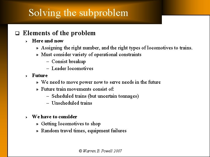
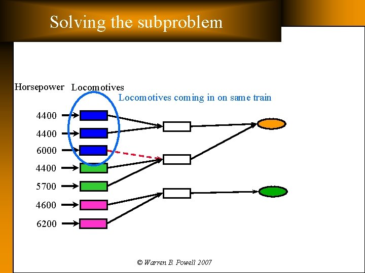
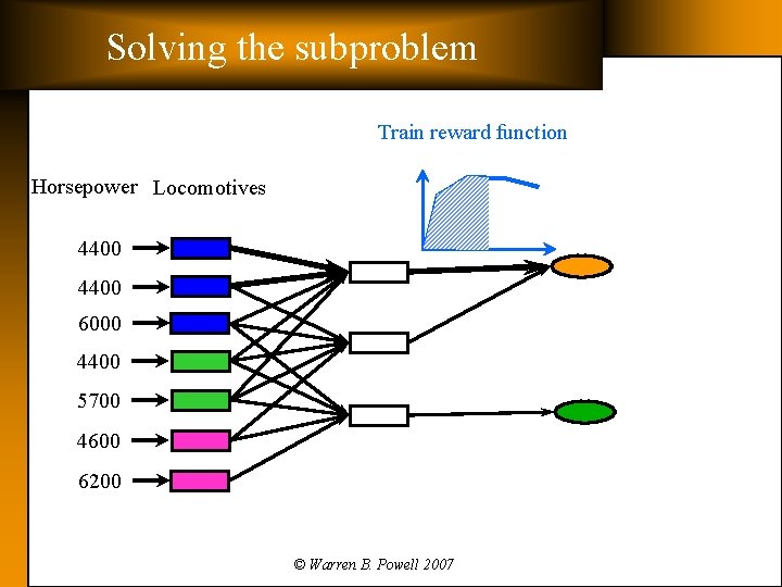
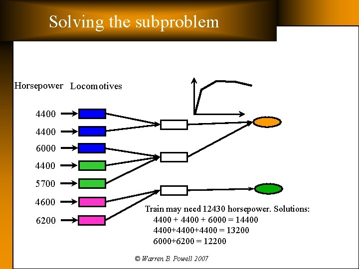
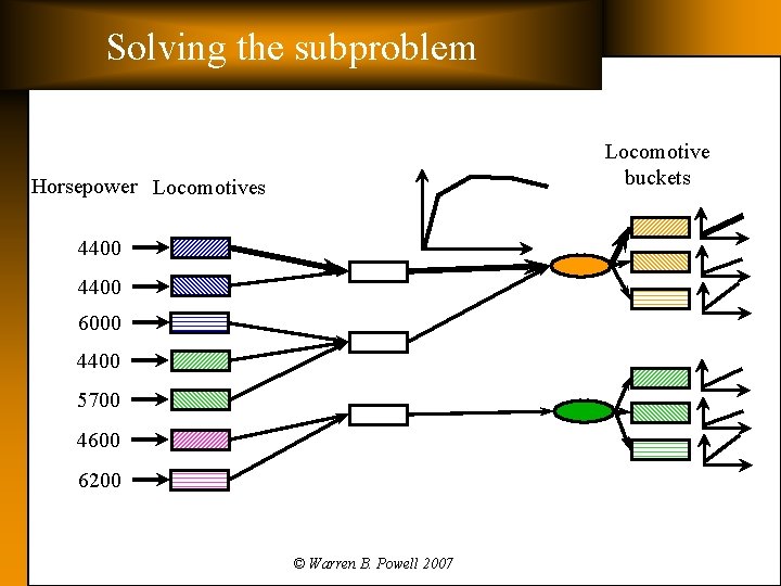
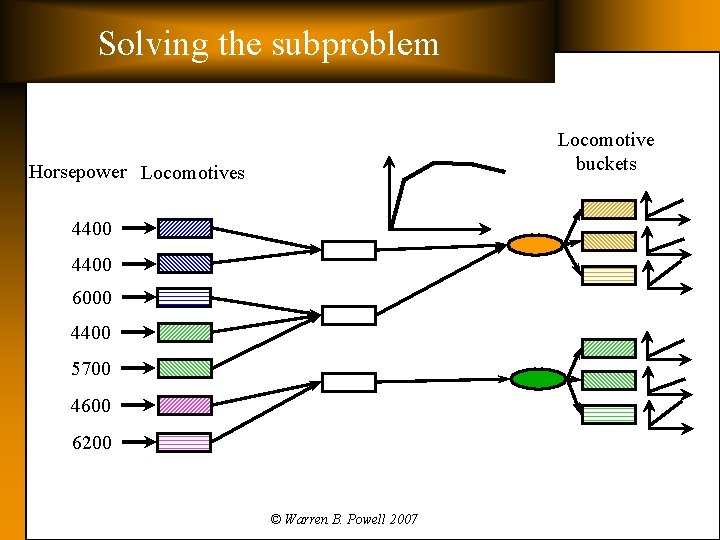
Solving the subproblem q Elements of the problem Ø Ø Ø Here and now » Assigning the right number, and the right types of locomotives to trains. » Must consider variety of operational constraints – Consist breakup – Leader locomotives Future » We need to move power now to serve needs in the future » Future train movements consist of: – Scheduled trains (but uncertain tonnages) – Unscheduled trains We have to consider » Getting locomotives to shop » Random travel times, equipment failures © Warren B. Powell 2007

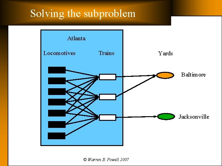
Solving the subproblem Atlanta Locomotives Trains Yards Baltimore Jacksonville © Warren B. Powell 2007

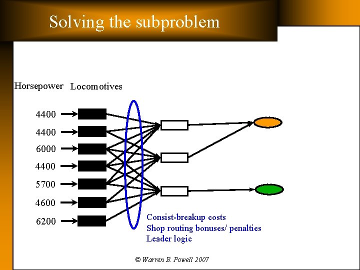
Solving the subproblem Horsepower Locomotives 4400 6000 4400 5700 4600 6200 Consist-breakup costs Shop routing bonuses/ penalties Leader logic © Warren B. Powell 2007

Solving the subproblem Horsepower Locomotives coming in on same train 4400 6000 4400 5700 4600 6200 © Warren B. Powell 2007

Solving the subproblem Train reward function Horsepower Locomotives 4400 6000 4400 5700 4600 6200 © Warren B. Powell 2007

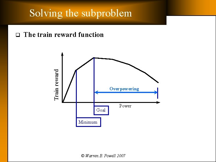
Solving the subproblem The train reward function Train reward q Overpowering Goal Power Minimum © Warren B. Powell 2007

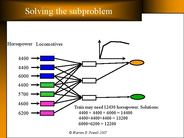
Solving the subproblem Horsepower Locomotives 4400 6000 4400 5700 4600 6200 Train may need 12430 horsepower. Solutions: 4400 + 6000 = 14400+4400 = 13200 6000+6200 = 12200 © Warren B. Powell 2007

Solving the subproblem Horsepower Locomotives 4400 6000 4400 5700 4600 6200 Train may need 12430 horsepower. Solutions: 4400 + 6000 = 14400+4400 = 13200 6000+6200 = 12200 © Warren B. Powell 2007

Solving the subproblem Locomotive buckets Horsepower Locomotives 4400 6000 4400 5700 4600 6200 © Warren B. Powell 2007

© Warren B. Powell 2007 43

© Warren B. Powell 2007 44

© Warren B. Powell 2007 45

© Warren B. Powell 2007 46

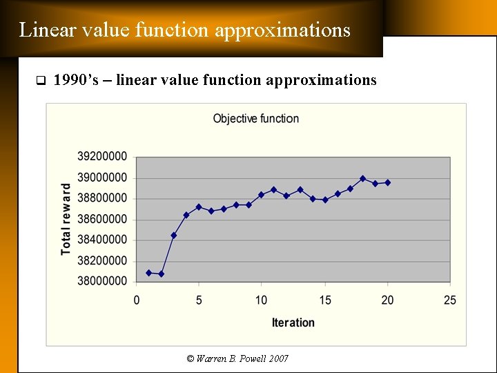
Linear value function approximations q 1990’s – linear value function approximations © Warren B. Powell 2007

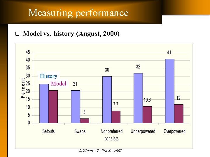
Measuring performance q Model vs. history (August, 2000) History Model © Warren B. Powell 2007

Results from the 1990’s q 1990’s Ø Ø q Solving locomotive assignment problem using a hybrid LP-relaxation and local search heuristic Value of locomotives in the future we estimated using linear functions Slope of the value function were estimated using the dual variable from the LP relaxation. Implemented in production at Norfolk Southern 2001 -2002. Weaknesses: Ø Ø Linear value function approximations could be unstable. Local search heuristic would occasionally produce “anomalies. ” » The fact that the solution was “not as good” was irrelevant. » Anomalies reduced confidence in the model. » Produced diagnostic problems, since it was not easy to identify why an odd locomotive assignment was due to data problem, model problem, coding issue, or the heuristic. © Warren B. Powell 2007

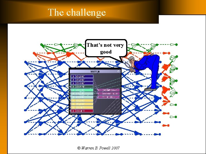
The challenge That’s not very good © Warren B. Powell 2007

Solving the subproblem Locomotive buckets Horsepower Locomotives 4400 6000 4400 5700 4600 6200 © Warren B. Powell 2007

Solving the subproblem Locomotive buckets Horsepower Locomotives 4400 6000 4400 5700 4600 6200 © Warren B. Powell 2007

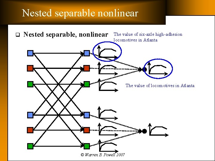
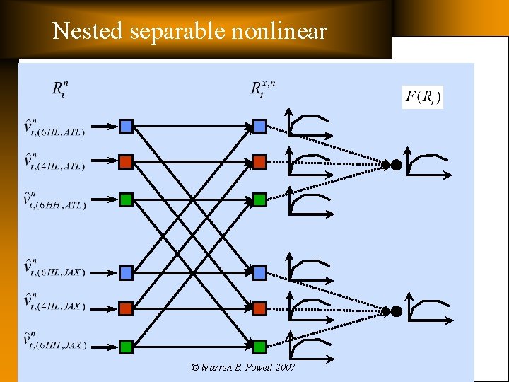
Status in 2007 q 2007: Ø Local search heuristic has been replaced with Cplex. » We have no trouble solving the IP to optimality, without sacrificing our ability to handle all the operational constraints. Ø Value function approximations: » First replaced linear with piecewise linear separable – Separate PWL value function for each type of locomotive at each location. – Works much better than linear, but not well enough. Occasionally would move 5 locomotives to a location that needed 4. Ø Introduced nested, separable piecewise linear value function approximation. © Warren B. Powell 2007

Nested separable nonlinear q Nested separable, nonlinear The value of six-axle high-adhesion locomotives in Atlanta The value of locomotives in Atlanta © Warren B. Powell 2007

Nested separable nonlinear © Warren B. Powell 2007

Nested separable nonlinear © Warren B. Powell 2007

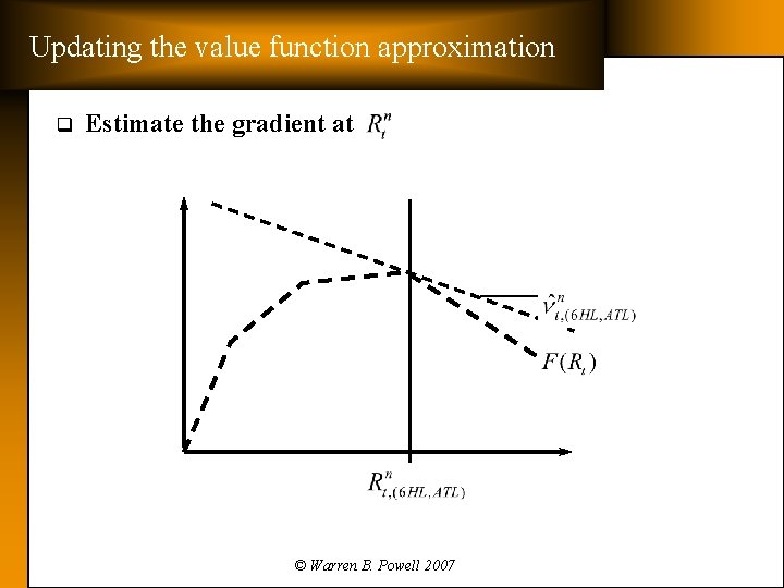
Updating the value function approximation q Estimate the gradient at © Warren B. Powell 2007

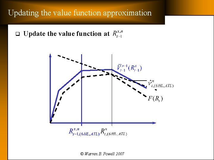
Updating the value function approximation q Update the value function at © Warren B. Powell 2007

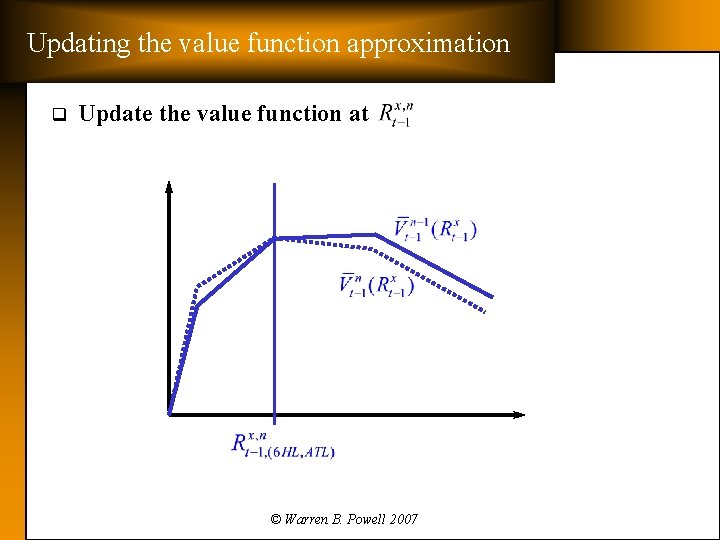
Updating the value function approximation q Update the value function at © Warren B. Powell 2007

Updating the value function approximation q Update the value function at © Warren B. Powell 2007

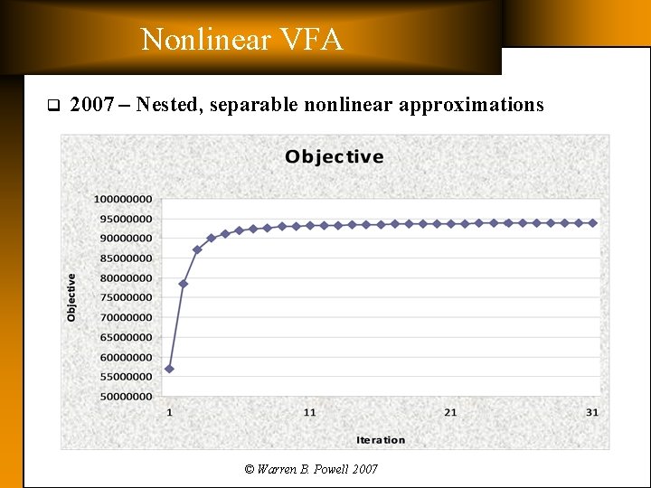
Nonlinear VFA q 2007 – Nested, separable nonlinear approximations © Warren B. Powell 2007

Outline q q q The locomotive planning problem Approximate dynamic programming Solving the subproblem Decomposition strategy Implementation © Warren B. Powell 2007

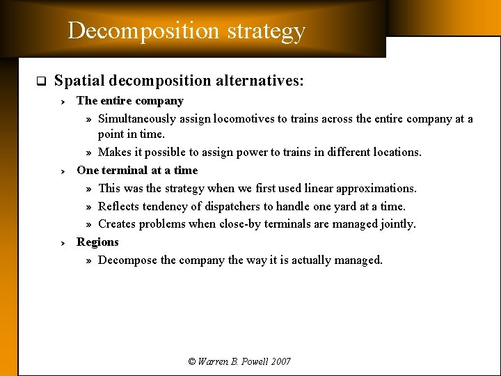
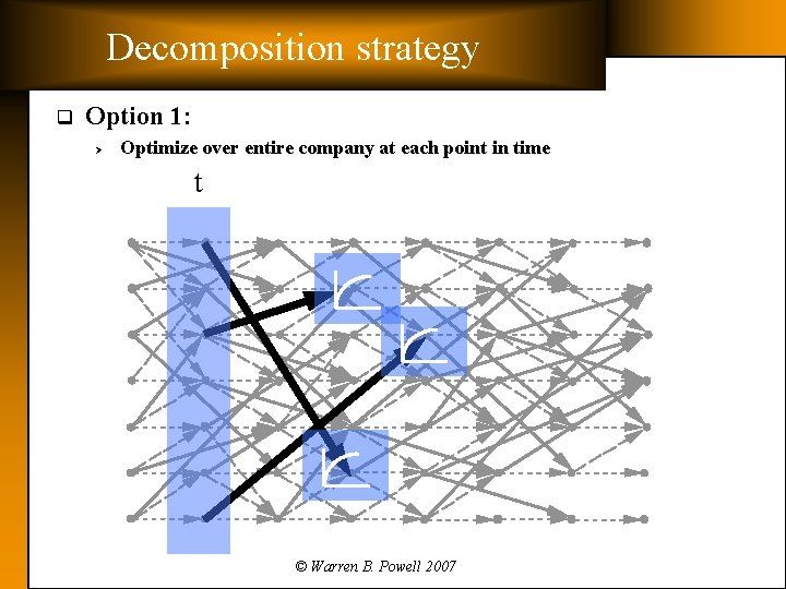
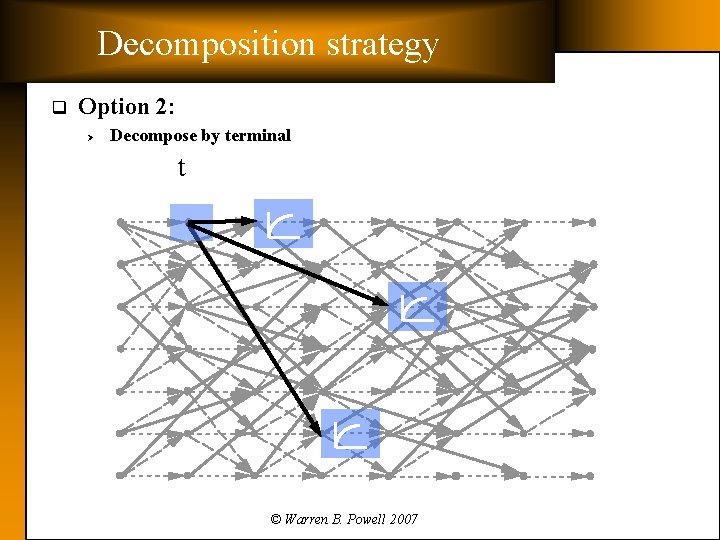
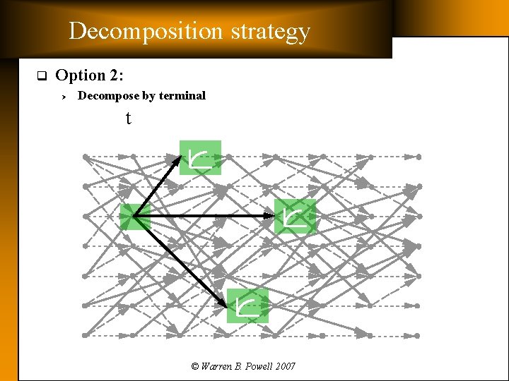
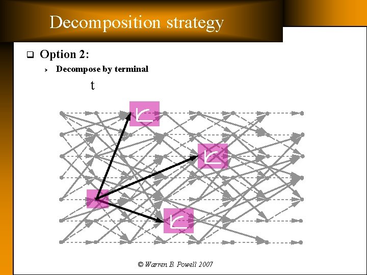
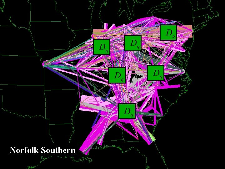
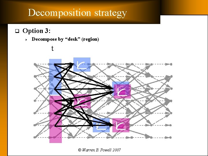
Decomposition strategy q Spatial decomposition alternatives: Ø Ø Ø The entire company » Simultaneously assign locomotives to trains across the entire company at a point in time. » Makes it possible to assign power to trains in different locations. One terminal at a time » This was the strategy when we first used linear approximations. » Reflects tendency of dispatchers to handle one yard at a time. » Creates problems when close-by terminals are managed jointly. Regions » Decompose the company the way it is actually managed. © Warren B. Powell 2007

Decomposition strategy q Option 1: Ø Optimize over entire company at each point in time t © Warren B. Powell 2007

Decomposition strategy q Option 2: Ø Decompose by terminal t © Warren B. Powell 2007

Decomposition strategy q Option 2: Ø Decompose by terminal t © Warren B. Powell 2007

Decomposition strategy q Option 2: Ø Decompose by terminal t © Warren B. Powell 2007

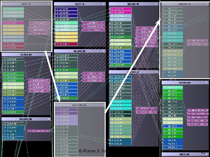
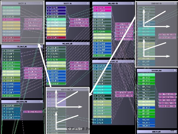
Norfolk Southern © Warren B. Powell 2007 68

© Warren B. Powell 2007

Decomposition strategy q Option 3: Ø Decompose by “desk” (region) t © Warren B. Powell 2007

Outline q q q The locomotive planning problem Approximate dynamic programming Solving the subproblem Decomposition strategy Implementation © Warren B. Powell 2007

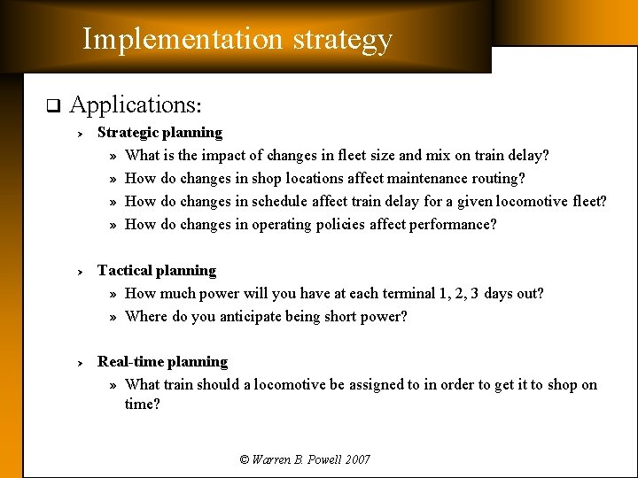
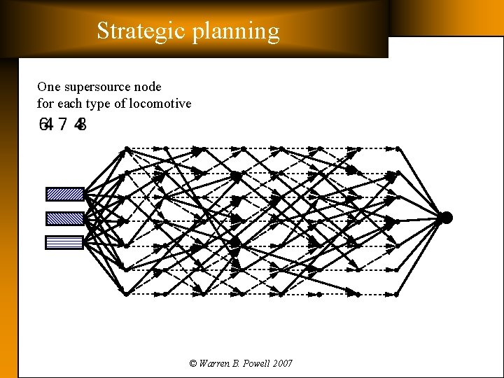
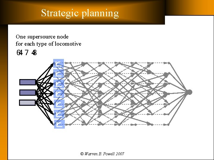
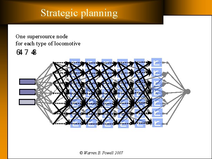
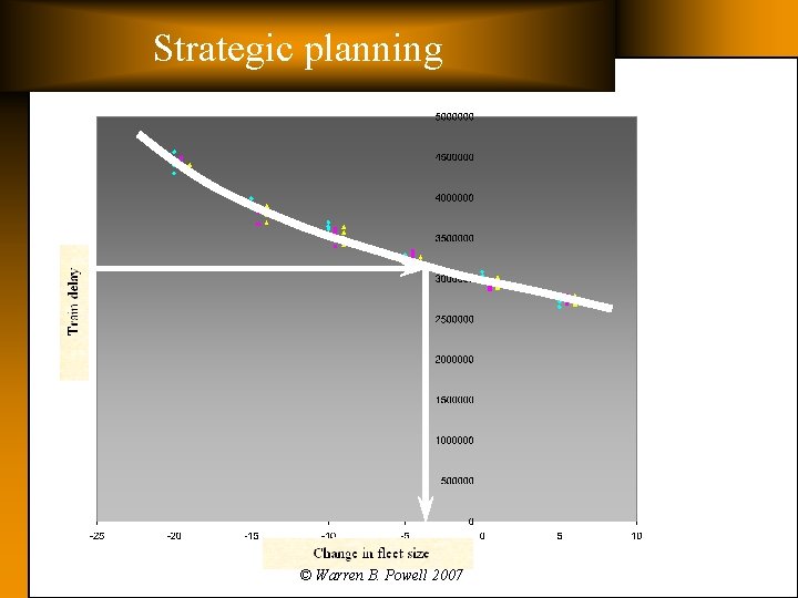
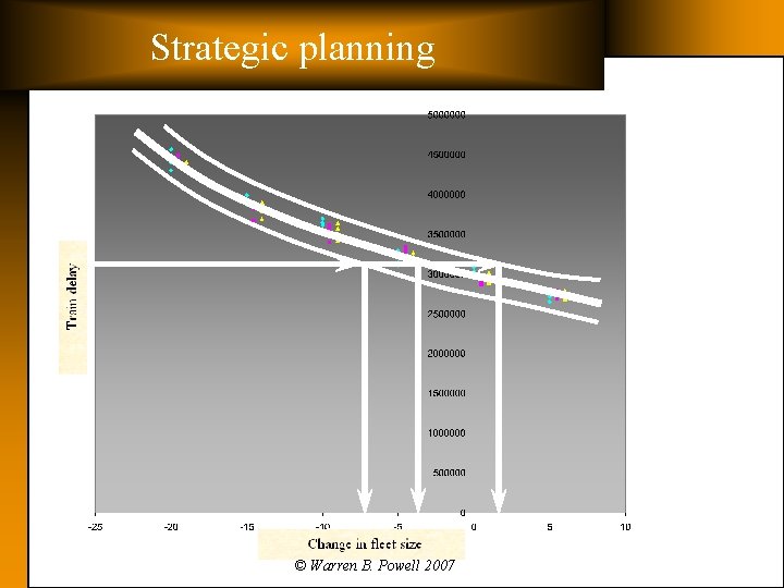
Implementation strategy q Applications: Ø Ø Ø Strategic planning » What is the impact of changes in fleet size and mix on train delay? » How do changes in shop locations affect maintenance routing? » How do changes in schedule affect train delay for a given locomotive fleet? » How do changes in operating policies affect performance? Tactical planning » How much power will you have at each terminal 1, 2, 3 days out? » Where do you anticipate being short power? Real-time planning » What train should a locomotive be assigned to in order to get it to shop on time? © Warren B. Powell 2007

Strategic planning One supersource node for each type of locomotive © Warren B. Powell 2007

Strategic planning One supersource node for each type of locomotive © Warren B. Powell 2007

Strategic planning One supersource node for each type of locomotive © Warren B. Powell 2007

Strategic planning One supersource node for each type of locomotive © Warren B. Powell 2007

Strategic planning One supersource node for each type of locomotive © Warren B. Powell 2007

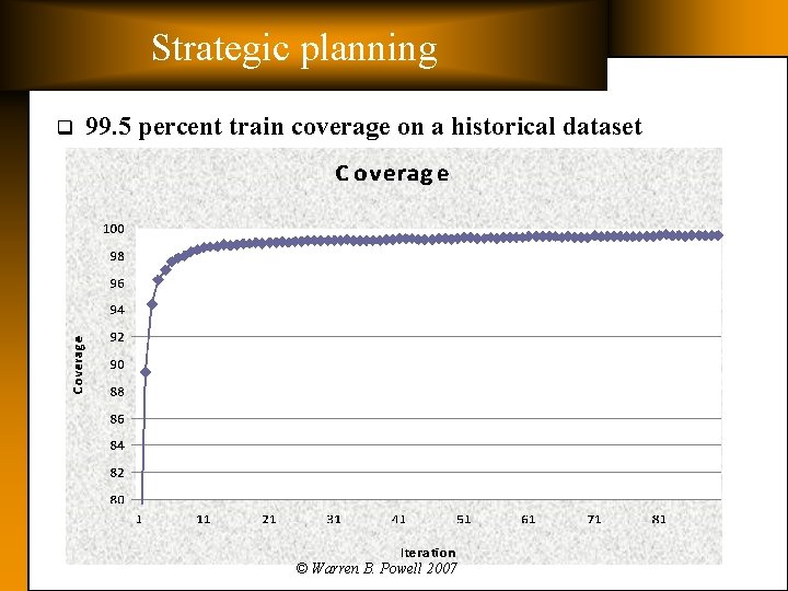
Strategic planning q 99. 5 percent train coverage on a historical dataset © Warren B. Powell 2007

Strategic planning © Warren B. Powell 2007

Strategic planning © Warren B. Powell 2007

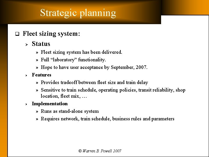
Strategic planning q Fleet sizing system: Ø Status » Fleet sizing system has been delivered. » Full “laboratory” functionality. » Hope to have user acceptance by September, 2007. Ø Ø Features » Provides tradeoff between fleet size and train delay » Sensitive to train schedule, operating policies, transit reliability, shop location, fleet mix, … Implementation » Runs as stand-alone system » Requires network, train schedule, business rules and parameters © Warren B. Powell 2007

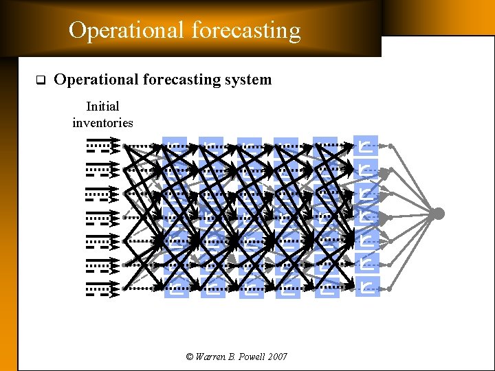
Operational forecasting q Operational forecasting system Initial inventories © Warren B. Powell 2007

Operational forecasting q Operational forecasting system Initial inventories © Warren B. Powell 2007

Operational forecasting q Operational forecasting system: Ø Status » Extensive calibration as part of the fleet sizing system. » Project will start fall, 2007. Ø Ø Features » Updates every 1 -2 minutes. » Models locomotives and trains at a high level of detail » Able to incorporate uncertainty into forecasts of train movements, tonnages and transit times » Uses same core model as the strategic planning system Implementation » Not yet started. » Sensitive issues: – Accuracy of locomotive snapshot – Ability to model unscheduled trains – Balancing user expectations for the accuracy of the forecast with the realities of messy railroad operations © Warren B. Powell 2007

Real-time locomotive assignment q Real-time system: Ø Status » Requires reoptimizing a single subproblem in real-time » Project will start summer, 2008. Ø Ø Features » Estimated reoptimization time for one subproblem < 1 second. » Responds in real-time to user overrides » Subproblem “talks” to operational planning model Implementation » Not yet started. » Sensitive issues: – Tight integration with existing user interface © Warren B. Powell 2007

pf © Warren B. Powell 2007