Applied Statistics with R Chapter 0 Statistics Basics

Applied Statistics with R Chapter 0. Statistics Basics Disclaimer: • All images such as logos, photos, etc. used in this presentation are the property of their respective copyright owners and are used here for educational purposes only • Case inspired by actual student presentation in analytics class; names withheld for privacy © Stephan Sorger 2017: www. stephansorger. com

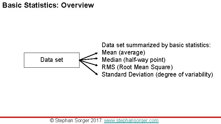
Basic Statistics: Overview Data set summarized by basic statistics: Mean (average) Median (half-way point) RMS (Root Mean Square) Standard Deviation (degree of variability) © Stephan Sorger 2017: www. stephansorger. com

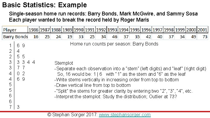
Basic Statistics: Example Single-season home run records: Barry Bonds, Mark Mc. Gwire, and Sammy Sosa Each player wanted to break the record held by Roger Maris 1 2 2 3 3 4 4 5 5 6 6 7 6 4 5 3 7 0 6 9 5 3 4 4 7 2 9 Home run counts per season: Barry Bonds Stemplot -Separate each observation into a “stem” (left digits) and “leaf” (right digit) So, 16 would be: 1 | 6 with “ 1” as the stem and “ 6” as the leaf -Write stems vertically in increasing order from top to bottom -Draw vertical line from top to bottom -”Split” the stems for greater clarity by entering two “ 2”, “ 3”, “ 4”, etc. -Interpret the stemplot: Study the distribution; Outlier at 73? 3 © Stephan Sorger 2017: www. stephansorger. com

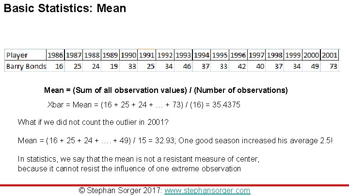
Basic Statistics: Mean = (Sum of all observation values) / (Number of observations) Xbar = Mean = (16 + 25 + 24 + … + 73) / (16) = 35. 4375 What if we did not count the outlier in 2001? Mean = (16 + 25 + 24 + …. + 49) / 15 = 32. 93; One good season increased his average 2. 5! In statistics, we say that the mean is not a resistant measure of center, because it cannot resist the influence of one extreme observation © Stephan Sorger 2017: www. stephansorger. com

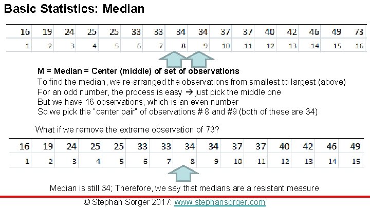
Basic Statistics: Median M = Median = Center (middle) of set of observations To find the median, we re-arranged the observations from smallest to largest (above) For an odd number, the process is easy just pick the middle one But we have 16 observations, which is an even number So we pick the “center pair” of observations # 8 and #9 (both of these are 34) What if we remove the extreme observation of 73? Median is still 34; Therefore, we say that medians are a resistant measure © Stephan Sorger 2017: www. stephansorger. com

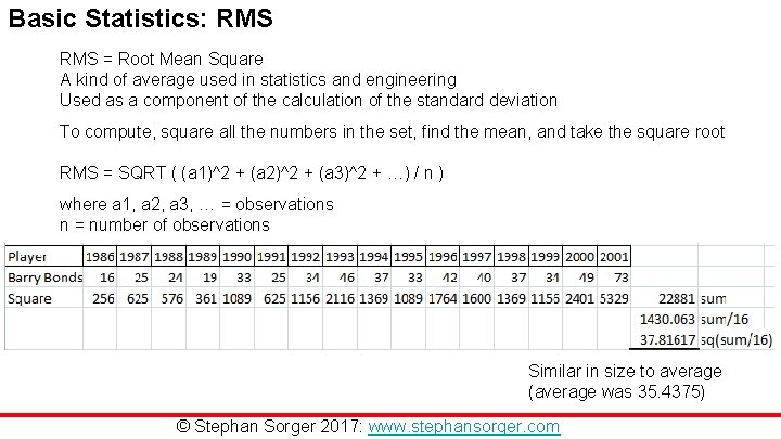
Basic Statistics: RMS = Root Mean Square A kind of average used in statistics and engineering Used as a component of the calculation of the standard deviation To compute, square all the numbers in the set, find the mean, and take the square root RMS = SQRT ( (a 1)^2 + (a 2)^2 + (a 3)^2 + …) / n ) where a 1, a 2, a 3, … = observations n = number of observations Similar in size to average (average was 35. 4375) © Stephan Sorger 2017: www. stephansorger. com

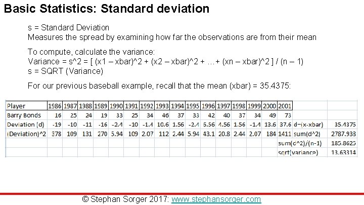
Basic Statistics: Standard deviation s = Standard Deviation Measures the spread by examining how far the observations are from their mean To compute, calculate the variance: Variance = s^2 = [ (x 1 – xbar)^2 + (x 2 – xbar)^2 + …+ (xn – xbar)^2 ] / (n – 1) s = SQRT (Variance) For our previous baseball example, recall that the mean (xbar) = 35. 4375: © Stephan Sorger 2017: www. stephansorger. com

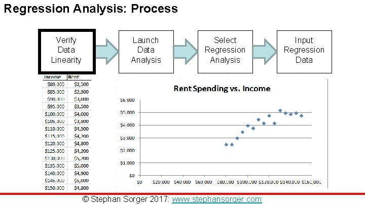
Regression Analysis: Process Verify Data Linearity Launch Data Analysis Select Regression Analysis © Stephan Sorger 2017: www. stephansorger. com Input Regression Data

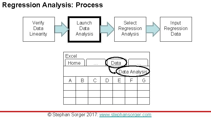
Regression Analysis: Process Verify Data Linearity Launch Data Analysis Excel Home Select Regression Analysis … Data Input Regression Data … Data Analysis A B C D E F G © Stephan Sorger 2017: www. stephansorger. com

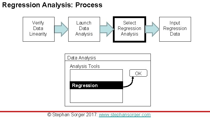
Regression Analysis: Process Verify Data Linearity Launch Data Analysis Select Regression Analysis Data Analysis Tools OK Regression © Stephan Sorger 2017: www. stephansorger. com Input Regression Data

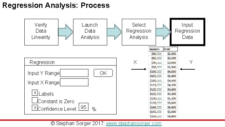
Regression Analysis: Process Verify Data Linearity Launch Data Analysis Select Regression Analysis Regression X Input Y Range OK Input X Range x Labels Constant is Zero x Confidence Level: 95 % © Stephan Sorger 2017: www. stephansorger. com Input Regression Data Y

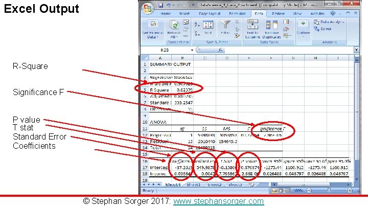
Excel Output R-Square Significance F P value T stat Standard Error Coefficients © Stephan Sorger 2017: www. stephansorger. com

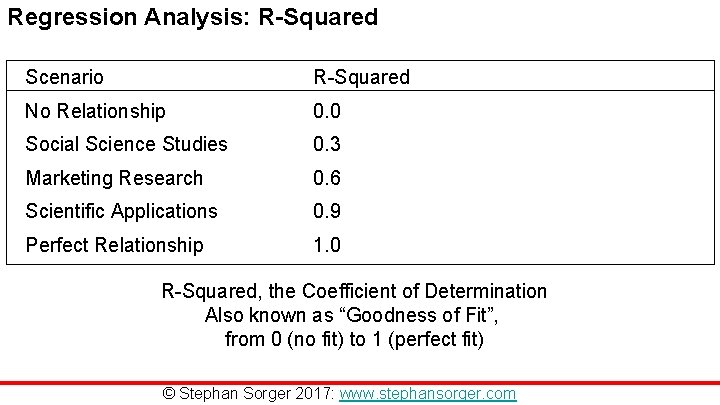
Regression Analysis: R-Squared Scenario R-Squared No Relationship 0. 0 Social Science Studies 0. 3 Marketing Research 0. 6 Scientific Applications 0. 9 Perfect Relationship 1. 0 R-Squared, the Coefficient of Determination Also known as “Goodness of Fit”, from 0 (no fit) to 1 (perfect fit) © Stephan Sorger 2017: www. stephansorger. com

Regression Analysis Testing © Stephan Sorger 2017: www. stephansorger. com

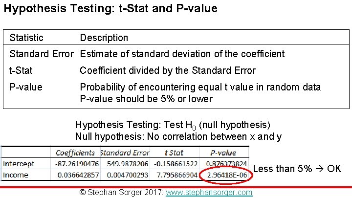
Hypothesis Testing: t-Stat and P-value Statistic Description Standard Error Estimate of standard deviation of the coefficient t-Stat Coefficient divided by the Standard Error P-value Probability of encountering equal t value in random data P-value should be 5% or lower Hypothesis Testing: Test H 0 (null hypothesis) Null hypothesis: No correlation between x and y Less than 5% OK © Stephan Sorger 2017: www. stephansorger. com

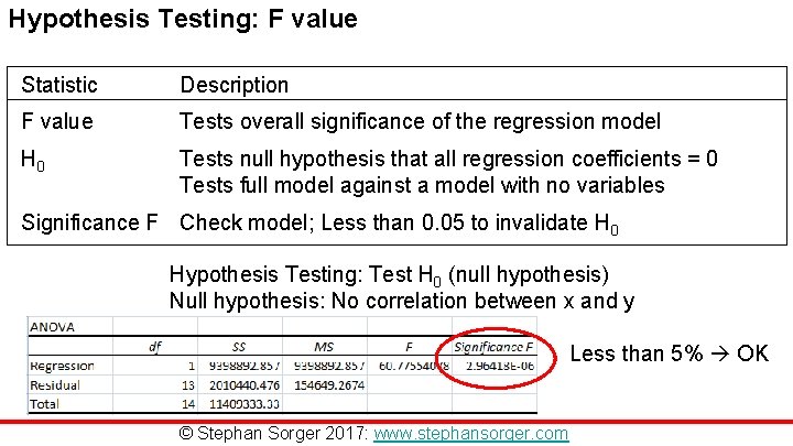
Hypothesis Testing: F value Statistic Description F value Tests overall significance of the regression model H 0 Tests null hypothesis that all regression coefficients = 0 Tests full model against a model with no variables Significance F Check model; Less than 0. 05 to invalidate H 0 Hypothesis Testing: Test H 0 (null hypothesis) Null hypothesis: No correlation between x and y Less than 5% OK © Stephan Sorger 2017: www. stephansorger. com

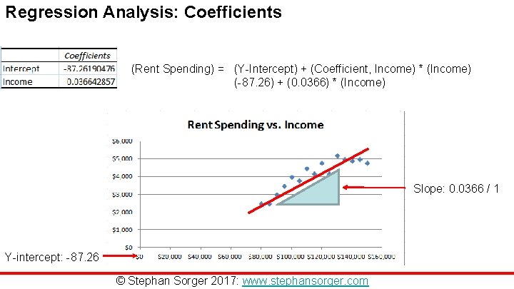
Regression Analysis: Coefficients (Rent Spending) = (Y-Intercept) + (Coefficient, Income) * (Income) (-87. 26) + (0. 0366) * (Income) Slope: 0. 0366 / 1 Y-intercept: -87. 26 © Stephan Sorger 2017: www. stephansorger. com

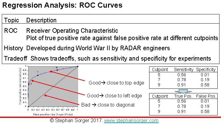
Regression Analysis: ROC Curves Topic Description ROC Receiver Operating Characteristic Plot of true positive rate against false positive rate at different cutpoints History Developed during World War II by RADAR engineers Tradeoff Shows tradeoffs, such as sensitivity and specificity for experiments Good close to top edge Good close to left edge Bad close to diagonal Cutpoint 5 7 9 Sensitivity Specificity 0. 56 0. 01 0. 78 0. 19 0. 91 0. 58 Cutpoint 5 7 9 True Pos. False Pos. 0. 56 0. 01 0. 78 0. 19 0. 91 0. 58 © Stephan Sorger 2017: www. stephansorger. com

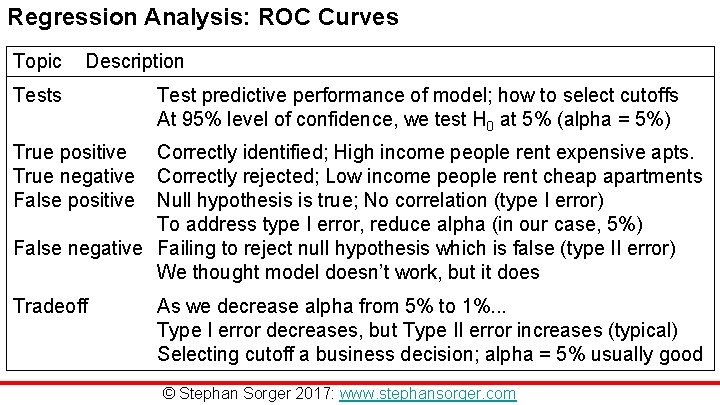
Regression Analysis: ROC Curves Topic Description Tests Test predictive performance of model; how to select cutoffs At 95% level of confidence, we test H 0 at 5% (alpha = 5%) True positive True negative False positive Correctly identified; High income people rent expensive apts. Correctly rejected; Low income people rent cheap apartments Null hypothesis is true; No correlation (type I error) To address type I error, reduce alpha (in our case, 5%) False negative Failing to reject null hypothesis which is false (type II error) We thought model doesn’t work, but it does Tradeoff As we decrease alpha from 5% to 1%. . . Type I error decreases, but Type II error increases (typical) Selecting cutoff a business decision; alpha = 5% usually good © Stephan Sorger 2017: www. stephansorger. com