Applied Statistics Outline Theoretical Lectures 2 5 hours

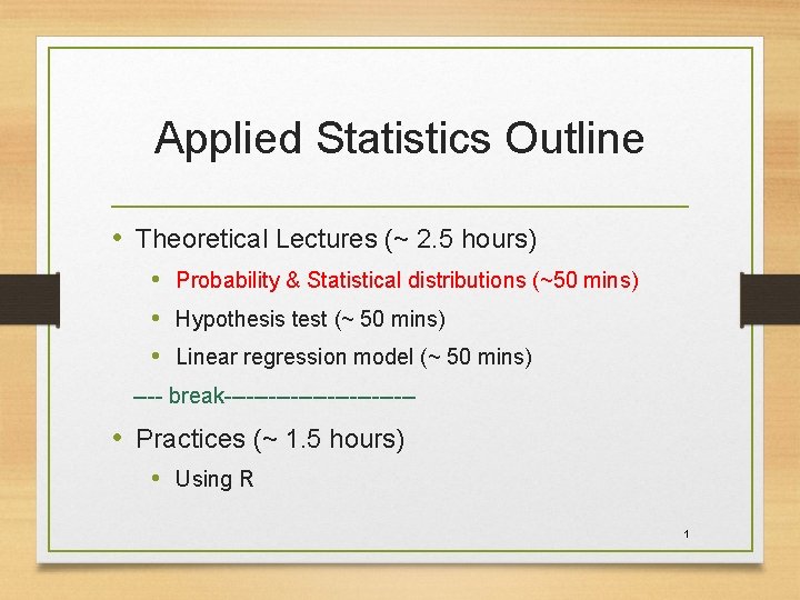
Applied Statistics Outline • Theoretical Lectures (~ 2. 5 hours) • Probability & Statistical distributions (~50 mins) • Hypothesis test (~ 50 mins) • Linear regression model (~ 50 mins) ---- break------------- • Practices (~ 1. 5 hours) • Using R 1

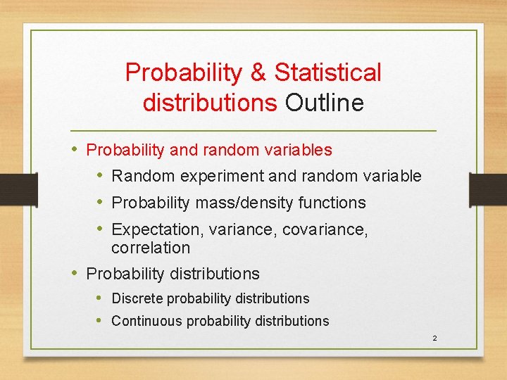
Probability & Statistical distributions Outline • Probability and random variables • Random experiment and random variable • Probability mass/density functions • Expectation, variance, correlation • Probability distributions • Discrete probability distributions • Continuous probability distributions 2

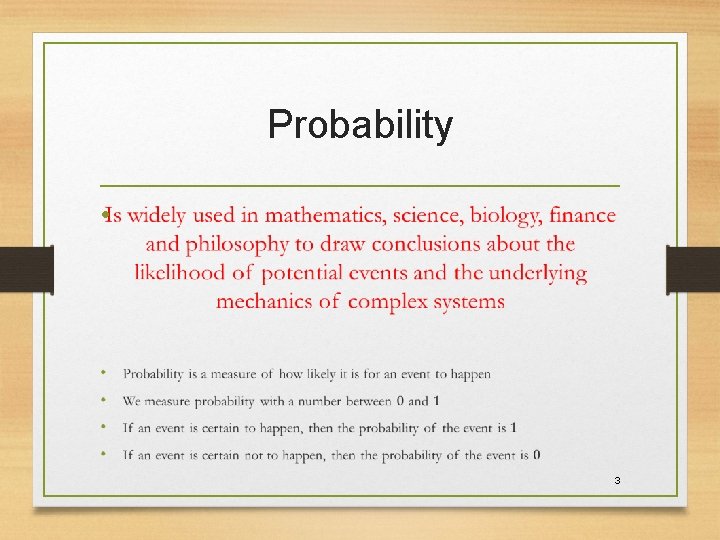
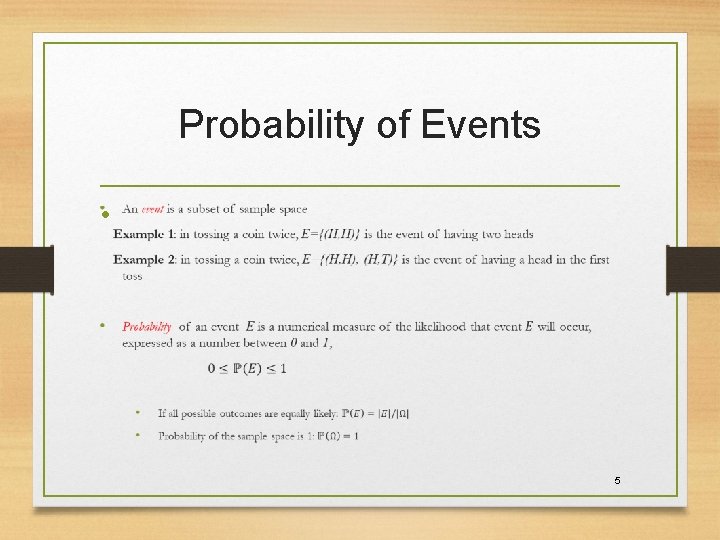
Probability • 3

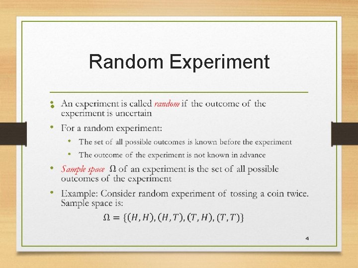
Random Experiment • 4

Probability of Events • 5

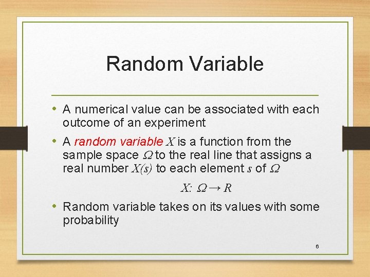
Random Variable • A numerical value can be associated with each outcome of an experiment • A random variable X is a function from the sample space to the real line that assigns a real number X(s) to each element s of X: → R • Random variable takes on its values with some probability 6

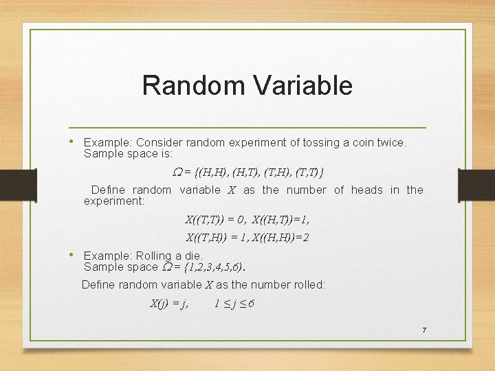
Random Variable • Example: Consider random experiment of tossing a coin twice. Sample space is: = {(H, H), (H, T), (T, H), (T, T)} Define random variable X as the number of heads in the experiment: X((T, T)) = 0, X((H, T))=1, X((T, H)) = 1, X((H, H))=2 • Example: Rolling a die. Sample space = {1, 2, 3, 4, 5, 6). Define random variable X as the number rolled: X(j) = j, 1≤j≤ 6 7

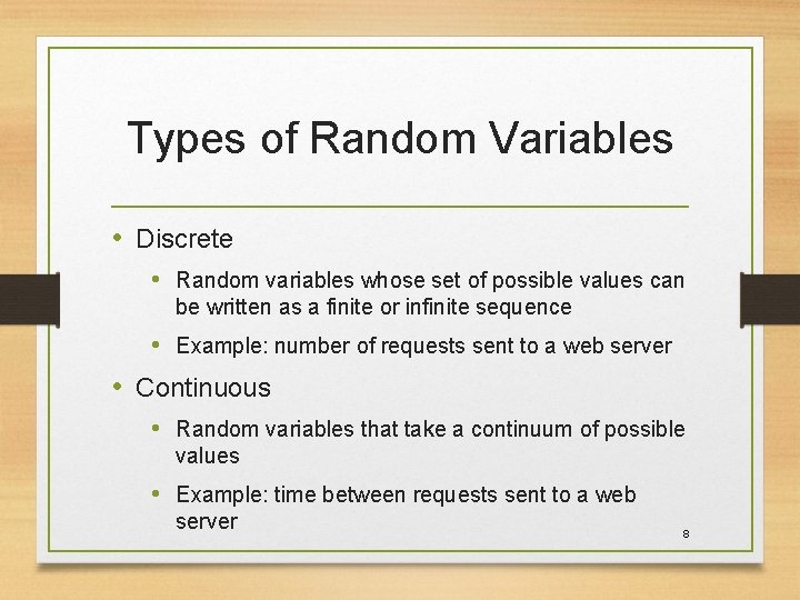
Types of Random Variables • Discrete • Random variables whose set of possible values can be written as a finite or infinite sequence • Example: number of requests sent to a web server • Continuous • Random variables that take a continuum of possible values • Example: time between requests sent to a web server 8

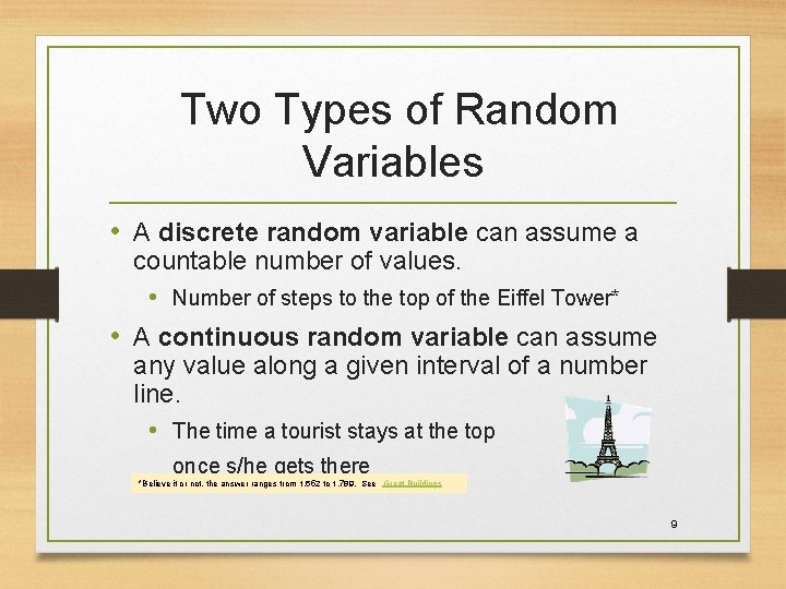
Two Types of Random Variables • A discrete random variable can assume a countable number of values. • Number of steps to the top of the Eiffel Tower* • A continuous random variable can assume any value along a given interval of a number line. • The time a tourist stays at the top once s/he gets there *Believe it or not, the answer ranges from 1, 652 to 1, 789. See Great Buildings 9

Two Types of Random Variables • Discrete random variables • Number of sales • Number of calls • Shares of stock • People in line • Mistakes per page • Continuous random variables • • • Length Depth Volume Time Weight 10

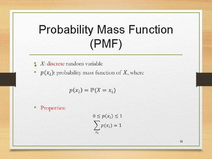
Probability Mass Function (PMF) • 13

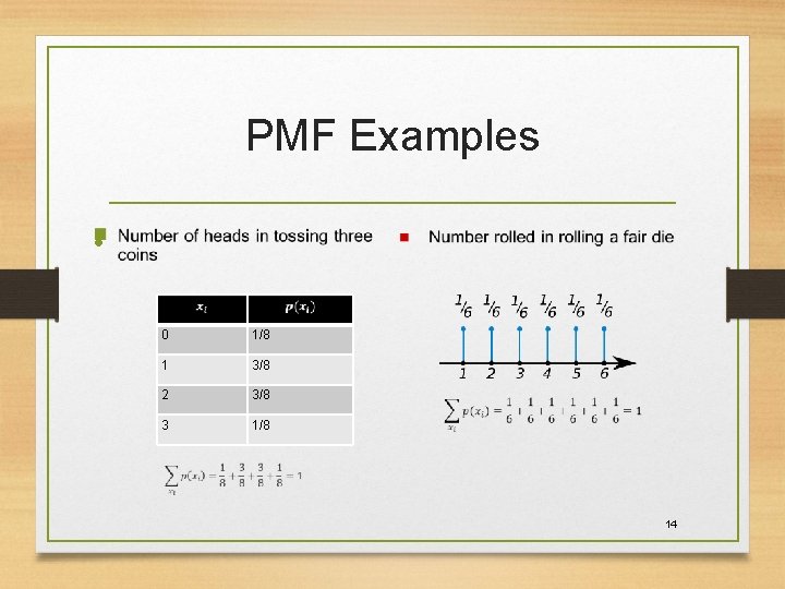
PMF Examples • 0 1/8 1 3/8 2 3/8 3 1/8 14

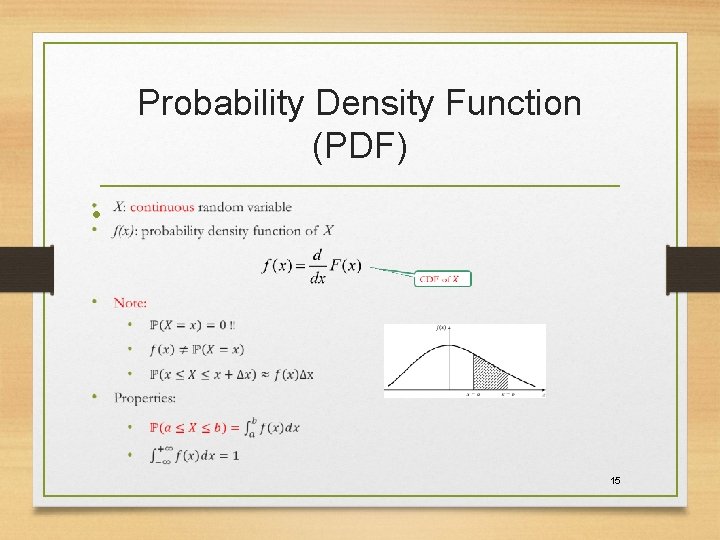
Probability Density Function (PDF) • 15

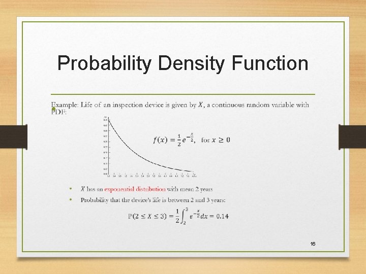
Probability Density Function • 16

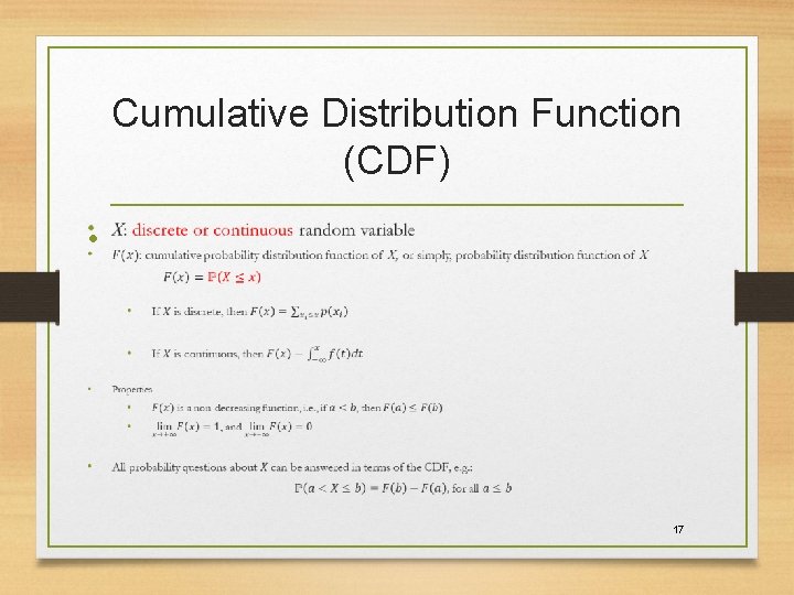
Cumulative Distribution Function (CDF) • 17

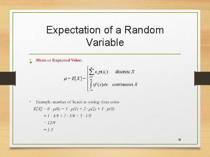
Expectation of a Random Variable • 18

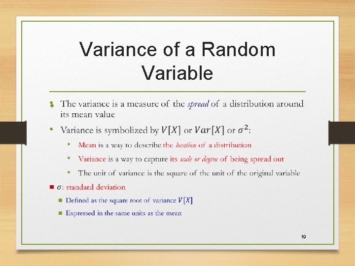
Variance of a Random Variable • 19

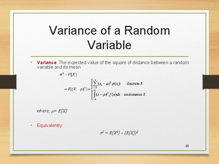
Variance of a Random Variable • Variance: The expected value of the square of distance between a random variable and its mean where, μ= E[X] • Equivalently: σ2 = E[X 2] – (E[X])2 20

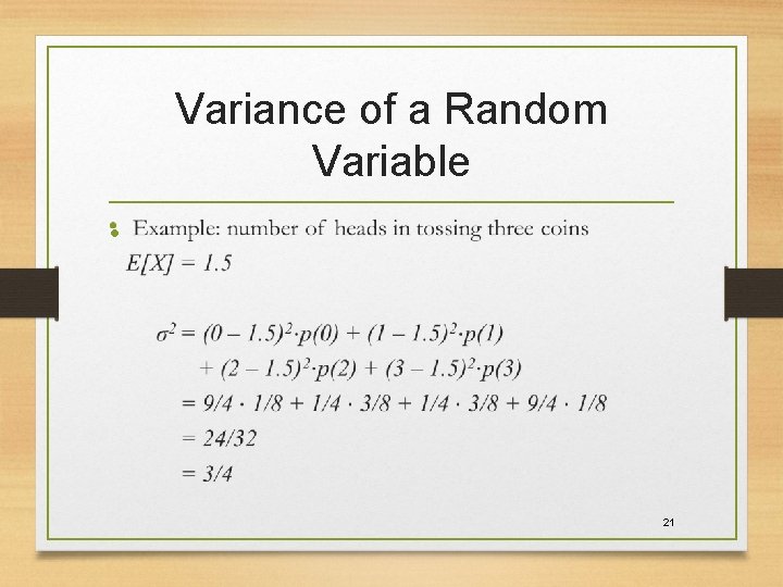
Variance of a Random Variable • 21

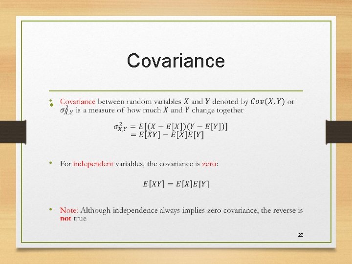
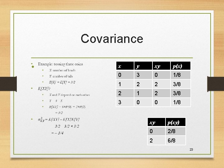
Covariance • 22

Covariance • x y xy p(x) 0 3 0 1/8 1 2 2 3/8 2 1 2 3/8 3 0 0 1/8 xy p(xy) 0 2/8 2 6/8 23

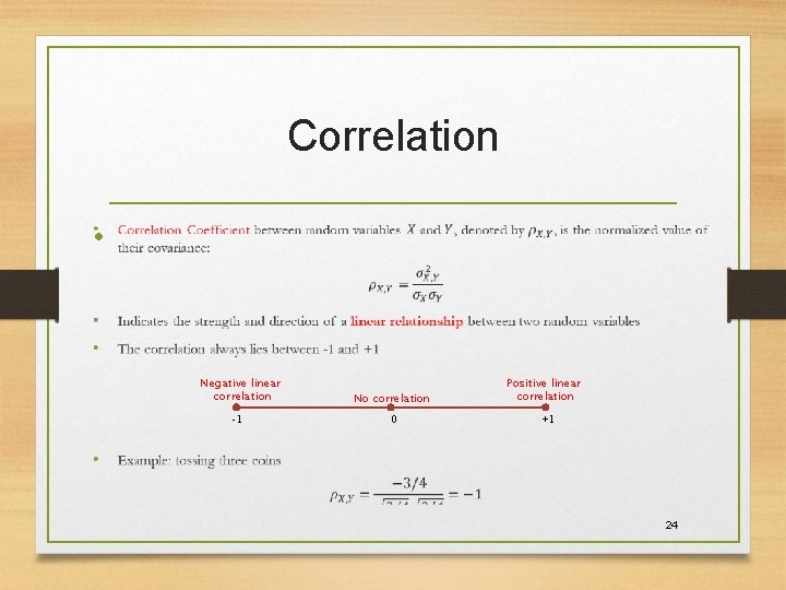
Correlation • Negative linear correlation -1 No correlation 0 Positive linear correlation +1 24

Probability & Statistical distributions Outline • Probability and random variables • Random experiment and random variable • Probability mass/density functions • Expectation, variance, correlation • Probability distributions • Discrete probability distributions • Continuous probability distributions 25

Outline • Probability and random variables • Random experiment and random variable • Probability mass/density functions • Expectation, variance, correlation • Probability distributions • Discrete probability distributions • Continuous probability distributions 26

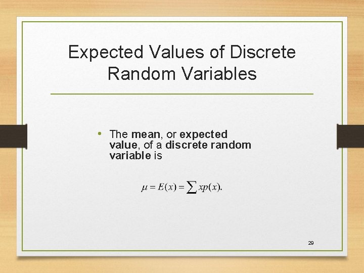
Expected Values of Discrete Random Variables • The mean, or expected value, of a discrete random variable is 29

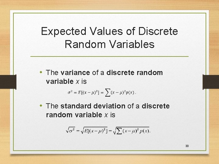
Expected Values of Discrete Random Variables • The variance of a discrete random variable x is • The standard deviation of a discrete random variable x is 30

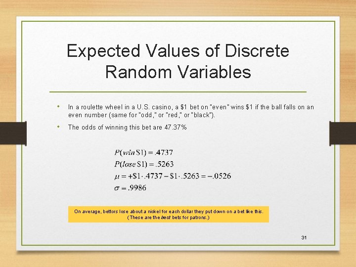
Expected Values of Discrete Random Variables • In a roulette wheel in a U. S. casino, a $1 bet on “even” wins $1 if the ball falls on an even number (same for “odd, ” or “red, ” or “black”). • The odds of winning this bet are 47. 37% On average, bettors lose about a nickel for each dollar they put down on a bet like this. (These are the best bets for patrons. ) 31

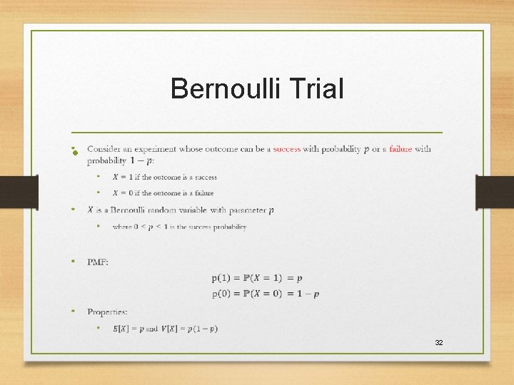
Bernoulli Trial • 32

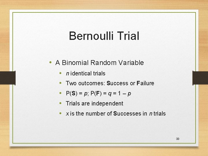
Bernoulli Trial • A Binomial Random Variable • • • n identical trials Two outcomes: Success or Failure P(S) = p; P(F) = q = 1 – p Trials are independent x is the number of Successes in n trials 33

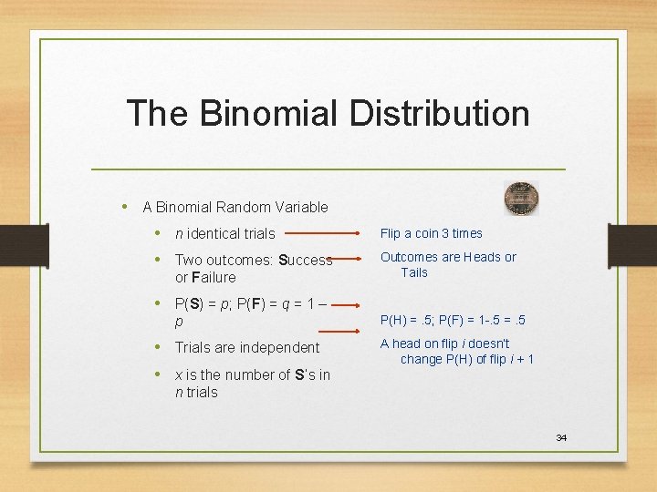
The Binomial Distribution • A Binomial Random Variable • n identical trials Flip a coin 3 times • Two outcomes: Success Outcomes are Heads or Tails or Failure • P(S) = p; P(F) = q = 1 – p • Trials are independent • x is the number of S’s in P(H) =. 5; P(F) = 1 -. 5 =. 5 A head on flip i doesn’t change P(H) of flip i + 1 n trials 34

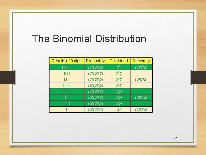
The Binomial Distribution Results of 3 flips Probability Combined Summary HHH (p)(p)(p) p 3 (1)p 3 q 0 HHT (p)(p)(q) p 2 q HTH (p)(q)(p) p 2 q THH (q)(p)(p) p 2 q HTT (p)(q)(q) pq 2 THT (q)(p)(q) pq 2 TTH (q)(q)(p) pq 2 TTT (q)(q)(q) q 3 (3)p 2 q 1 (3)p 1 q 2 (1)p 0 q 3 35

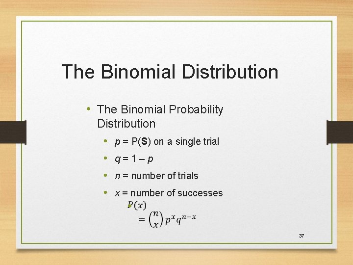
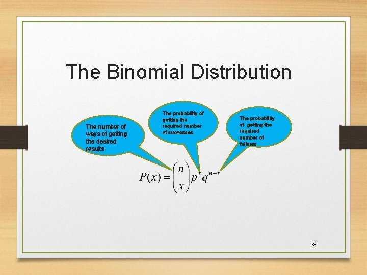
The Binomial Distribution • The Binomial Probability Distribution • p = P(S) on a single trial • q=1–p • n = number of trials • x = number of successes • 37

The Binomial Distribution The number of ways of getting the desired results The probability of getting the required number of successes The probability of getting the required number of failures 38

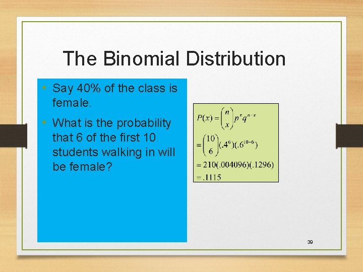
The Binomial Distribution • Say 40% of the class is female. • What is the probability that 6 of the first 10 students walking in will be female? 39

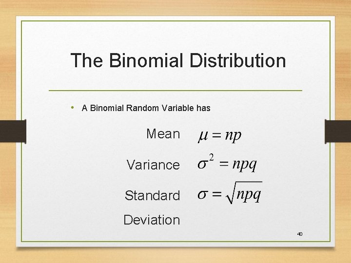
The Binomial Distribution • A Binomial Random Variable has Mean Variance Standard Deviation 40

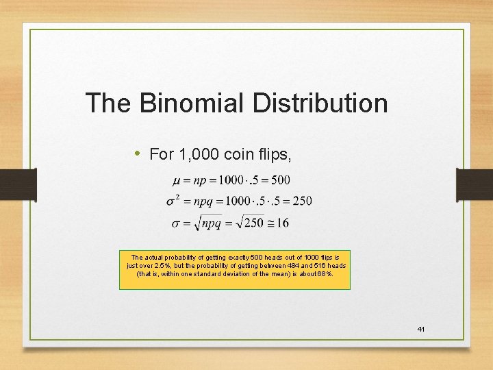
The Binomial Distribution • For 1, 000 coin flips, The actual probability of getting exactly 500 heads out of 1000 flips is just over 2. 5%, but the probability of getting between 484 and 516 heads (that is, within one standard deviation of the mean) is about 68%. 41

Poisson Distribution • Number of events occurring in a fixed time interval • Events occur with a known rate and are independent • Poisson distribution is characterized by the rate • Rate: the average number of event occurrences in a fixed time interval • Examples • The number of calls received by a switchboard per minute • The number of packets coming to a router per second • The number of travelers arriving to the airport for flight registration per hour 42

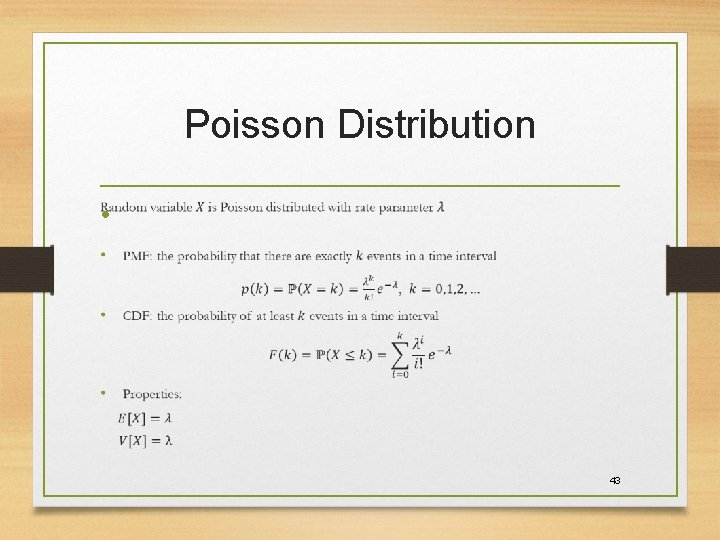
Poisson Distribution • 43

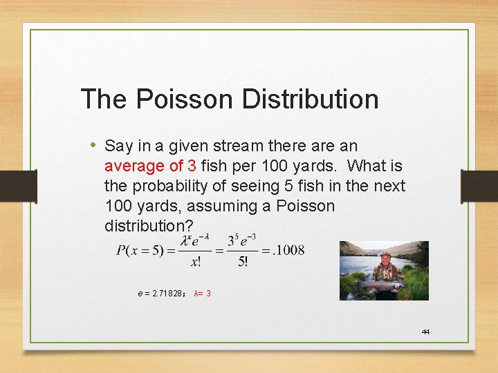
The Poisson Distribution • Say in a given stream there an average of 3 fish per 100 yards. What is the probability of seeing 5 fish in the next 100 yards, assuming a Poisson distribution? e = 2. 71828； λ= 3 44

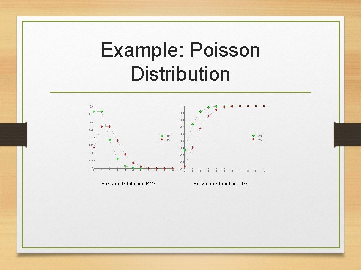
Example: Poisson Distribution Poisson distribution PMF Poisson distribution CDF

Outline • Probability and random variables • Random experiment and random variable • Probability mass/density functions • Expectation, variance, correlation • Probability distributions • Discrete probability distributions • Continuous probability distributions 47

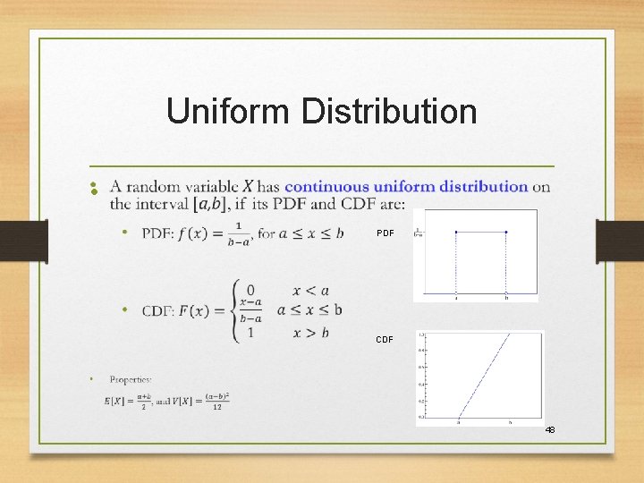
Uniform Distribution • PDF CDF 48

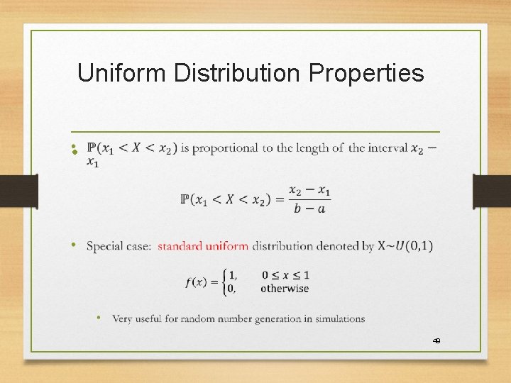
Uniform Distribution Properties • 49

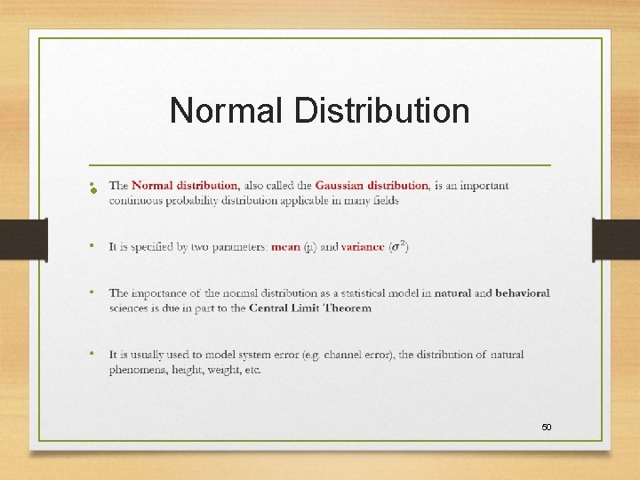
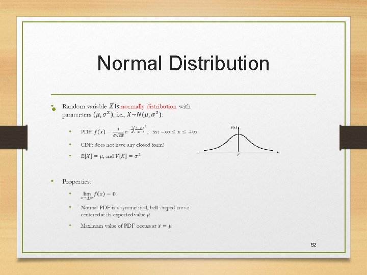
Normal Distribution • 50

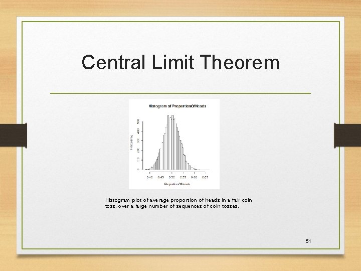
Central Limit Theorem Histogram plot of average proportion of heads in a fair coin toss, over a large number of sequences of coin tosses. 51

Normal Distribution • 52

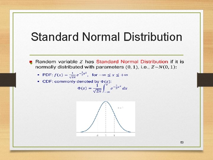
Standard Normal Distribution • 53

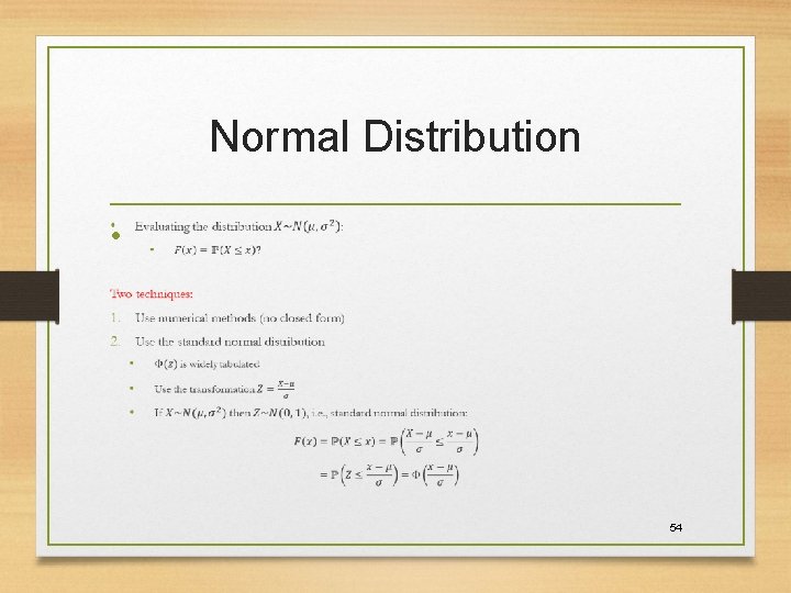
Normal Distribution • 54

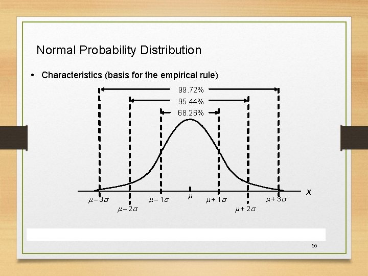
Normal Probability Distribution • Characteristics (basis for the empirical rule) 99. 72% 95. 44% 68. 26% – 3 s – 1 s – 2 s + 3 s + 1 s x + 2 s 55

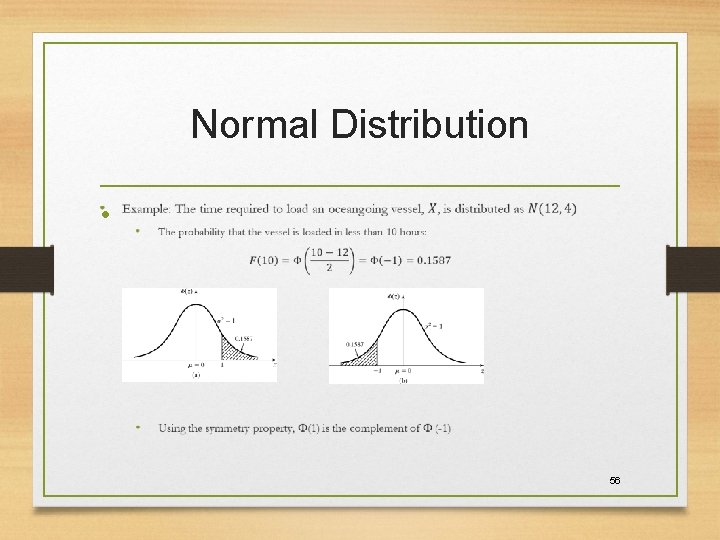
Normal Distribution • 56

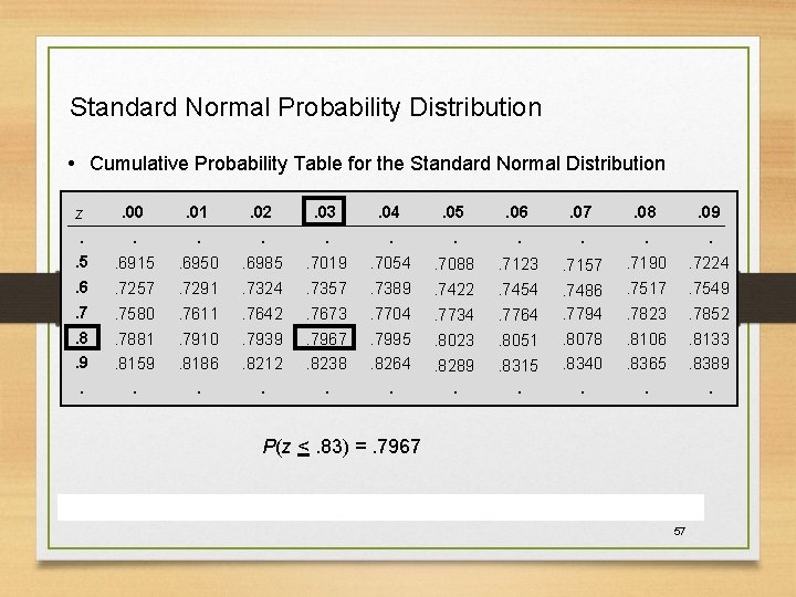
Standard Normal Probability Distribution • Cumulative Probability Table for the Standard Normal Distribution z. . 00 . 01 . 02 . 03 . 04 . 05 . 06 . 07 . 08 . 09 . . . 5 . 6915 . 6950 . 6985 . 7019 . 7054 . 7088 . 7123 . 7157 . 7190 . 7224 . 6 . 7257 . 7291 . 7324 . 7357 . 7389 . 7422 . 7454 . 7517 . 7549 . 7580 . 7611 . 7642 . 7673 . 7704 . 7734 . 7764 . 7486. 7794 . 7823 . 7852 . 8 . 7881 . 7910 . 7939 . 7967 . 7995 . 8023 . 8051 . 8078 . 8106 . 8133 . 9 . 8159. . 8186. . 8212. . 8238. . 8264. . 8289. . 8315. . 8340. . 8365. . 8389. . P(z <. 83) =. 7967 57

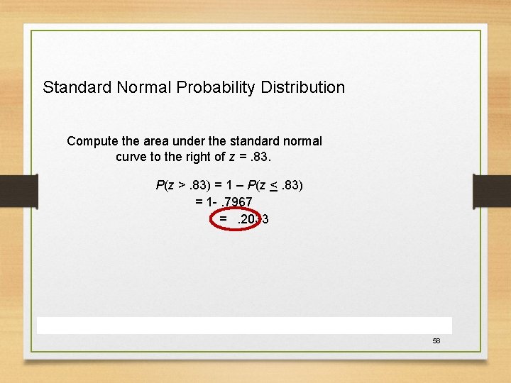
Standard Normal Probability Distribution Compute the area under the standard normal curve to the right of z =. 83. P(z >. 83) = 1 – P(z <. 83) = 1 -. 7967 =. 2033 58

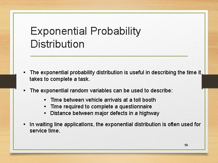
Exponential Probability Distribution • The exponential probability distribution is useful in describing the time it takes to complete a task. • The exponential random variables can be used to describe: • Time between vehicle arrivals at a toll booth • Time required to complete a questionnaire • Distance between major defects in a highway • In waiting line applications, the exponential distribution is often used for service time. 59

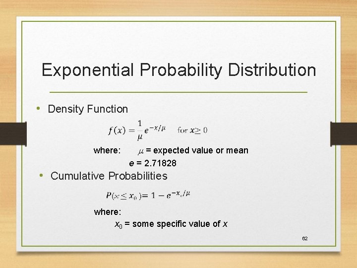
Exponential Probability Distribution • Density Function where: = expected value or mean e = 2. 71828 • Cumulative Probabilities where: x 0 = some specific value of x 62

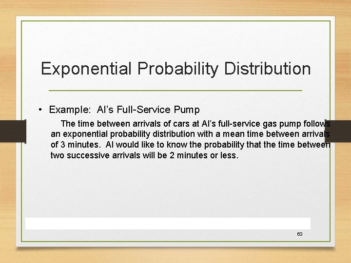
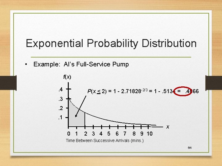
Exponential Probability Distribution • Example: Al’s Full-Service Pump The time between arrivals of cars at Al’s full-service gas pump follows an exponential probability distribution with a mean time between arrivals of 3 minutes. Al would like to know the probability that the time between two successive arrivals will be 2 minutes or less. 63

Exponential Probability Distribution • Example: Al’s Full-Service Pump f(x). 4 P(x < 2) = 1 - 2. 71828 -2/3 = 1 -. 5134 =. 4866 . 3. 2. 1 x 0 1 2 3 4 5 6 7 8 9 10 Time Between Successive Arrivals (mins. ) 64

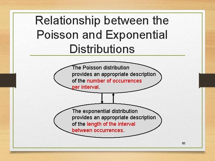
Relationship between the Poisson and Exponential Distributions The Poisson distribution provides an appropriate description of the number of occurrences per interval. The exponential distribution provides an appropriate description of the length of the interval between occurrences. 65

The Gamma Distribution and Its Relatives 66

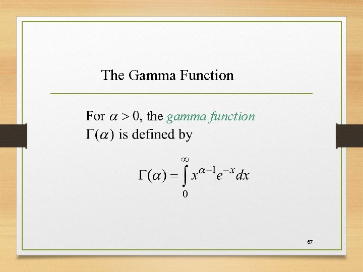
The Gamma Function the gamma function 67

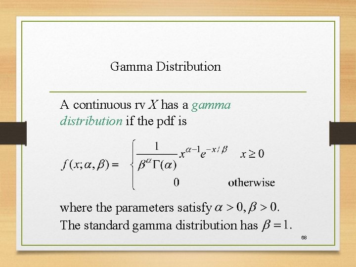
Gamma Distribution A continuous rv X has a gamma distribution if the pdf is where the parameters satisfy The standard gamma distribution has 68

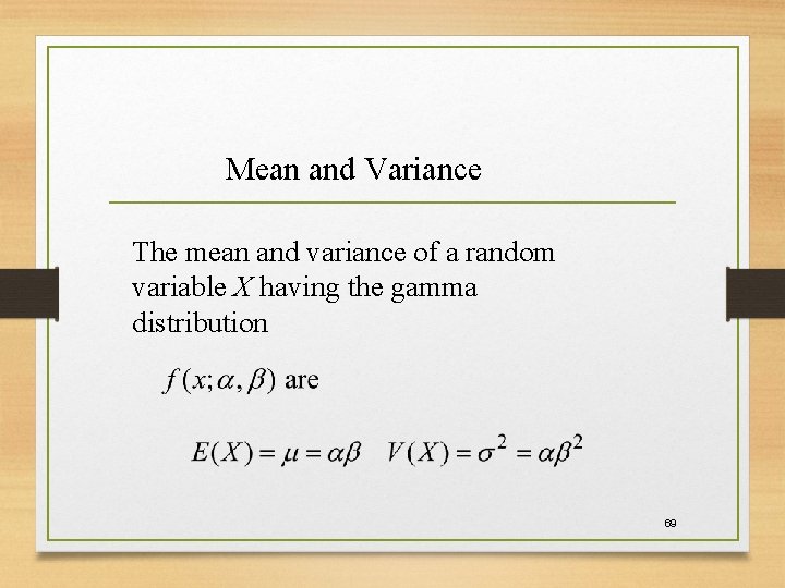
Mean and Variance The mean and variance of a random variable X having the gamma distribution 69

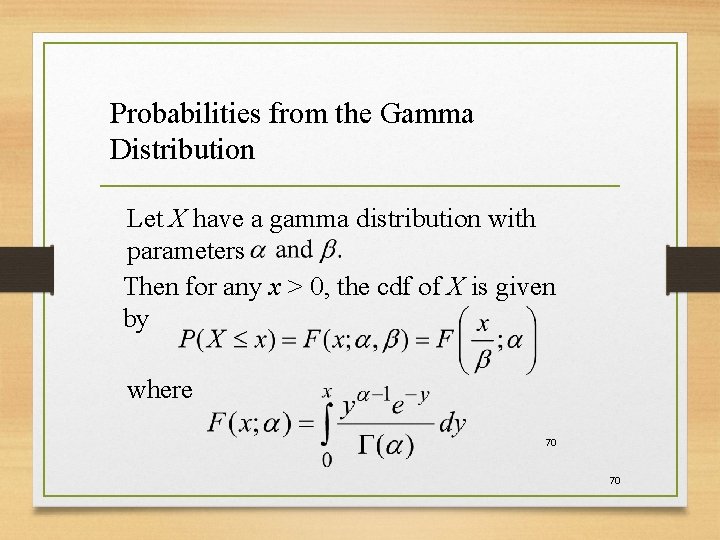
Probabilities from the Gamma Distribution Let X have a gamma distribution with parameters Then for any x > 0, the cdf of X is given by where 70 70

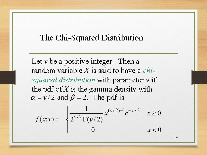
The Chi-Squared Distribution Let v be a positive integer. Then a random variable X is said to have a chisquared distribution with parameter v if the pdf of X is the gamma density with The pdf is 71

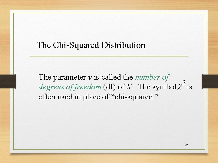
The Chi-Squared Distribution The parameter v is called the number of degrees of freedom (df) of X. The symbol often used in place of “chi-squared. ” is 72

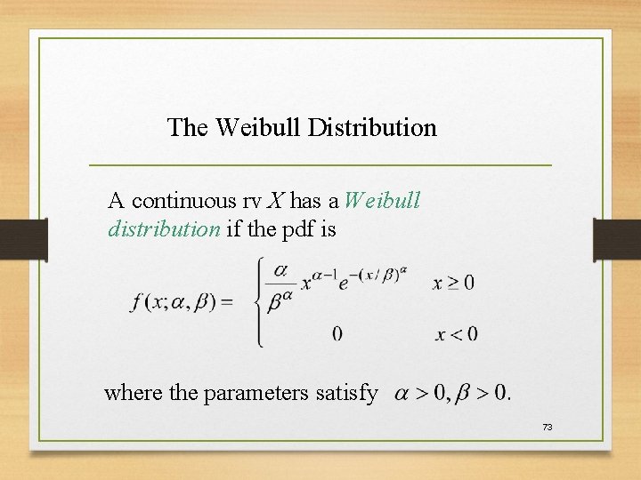
The Weibull Distribution A continuous rv X has a Weibull distribution if the pdf is where the parameters satisfy 73

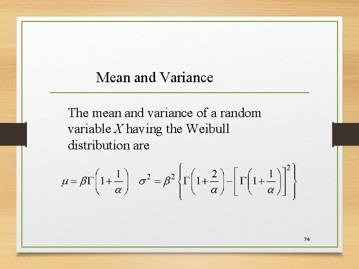
Mean and Variance The mean and variance of a random variable X having the Weibull distribution are 74

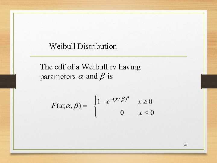
Weibull Distribution The cdf of a Weibull rv having parameters 75

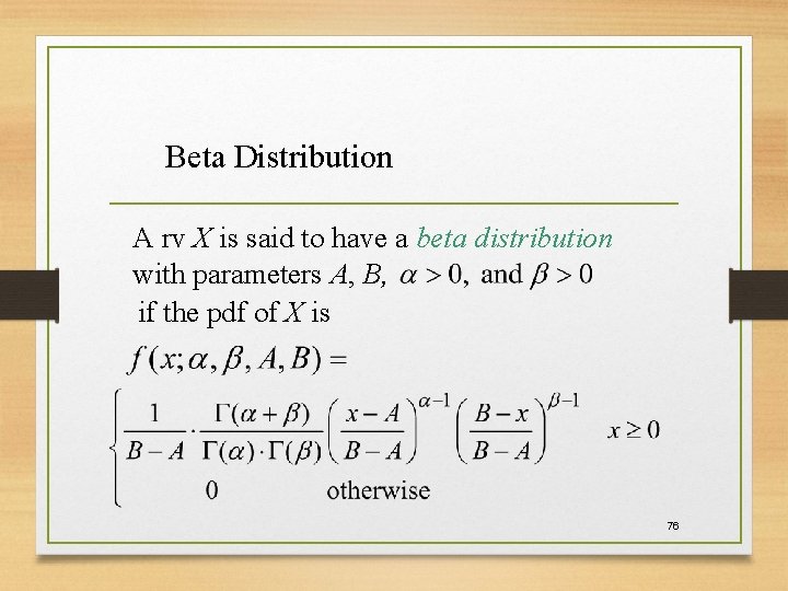
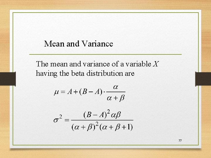
Beta Distribution A rv X is said to have a beta distribution with parameters A, B, if the pdf of X is 76

Mean and Variance The mean and variance of a variable X having the beta distribution are 77