Applied Risk Analytics Making Advanced Analytics More Useful

Applied Risk Analytics: Making Advanced Analytics More Useful Tony Cox tcoxdenver@aol. com NPS August 4, 2016

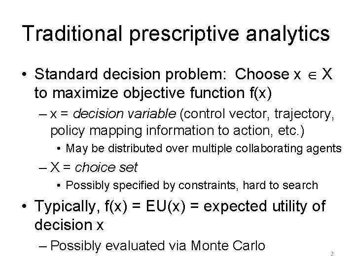
Traditional prescriptive analytics • Standard decision problem: Choose x X to maximize objective function f(x) – x = decision variable (control vector, trajectory, policy mapping information to action, etc. ) • May be distributed over multiple collaborating agents – X = choice set • Possibly specified by constraints, hard to search • Typically, f(x) = EU(x) = expected utility of decision x – Possibly evaluated via Monte Carlo 2

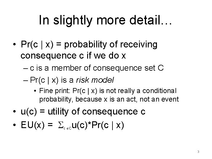
In slightly more detail… • Pr(c | x) = probability of receiving consequence c if we do x – c is a member of consequence set C – Pr(c | x) is a risk model • Fine print: Pr(c | x) is not really a conditional probability, because x is an act, not an event • u(c) = utility of consequence c • EU(x) = u(c)*Pr(c | x) c C 3

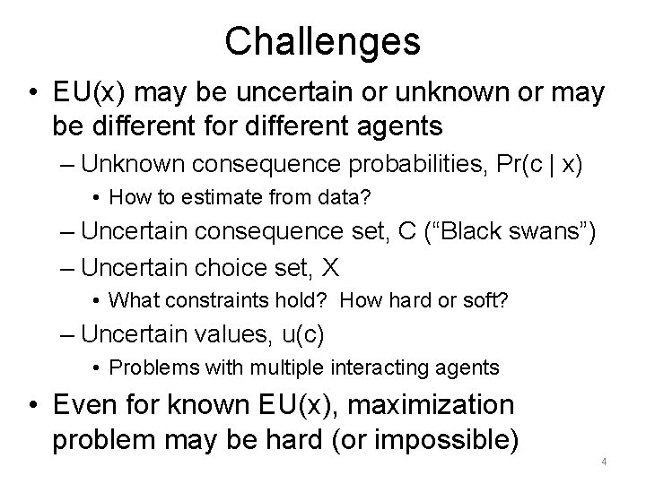
Challenges • EU(x) may be uncertain or unknown or may be different for different agents – Unknown consequence probabilities, Pr(c | x) • How to estimate from data? – Uncertain consequence set, C (“Black swans”) – Uncertain choice set, X • What constraints hold? How hard or soft? – Uncertain values, u(c) • Problems with multiple interacting agents • Even for known EU(x), maximization problem may be hard (or impossible) 4

Causal analysis challenge • What to do next when consequences of alternative decisions are uncertain? – Known probabilities → EU theory • Known risk model: Pr(c | x) • Known probabilities of different risk models – Unknown probabilities → ? 5

Decisions with unknown models • Learn causal model(s) from data/experience, then use them to optimize decisions – Design of experiments (DOE) – Randomized control trials (RCTs) and practical PCTs – Learn from natural experiments, quasi-experiments • Learn decision rules from data – Adaptive learning: trial and error, low-regret learning • Robust optimization – Find decisions that perform well no matter how uncertainties are resolved 6

Applied risk analytics toolkit: Toward more practical analytics Goal: Discover how to act more effectively 1. Descriptive analytics: What’s happening? 2. Predictive analytics: What’s coming next? 3. Causal analytics: What can we do about it? 4. Prescriptive analytics: What should we do? 5. Evaluation analytics: How well is it working? 6. Learning analytics: How to do better? 7. Collaboration: How to do better together? 7

Descriptive analytics: What’s going on? • What is the current situation? – Attribution: How many people per year are being killed (or harmed) by X? • Causes are often unobserved or uncertain • What has changed recently? (Why? ) – Example: More extreme event reports caused by real change or by media? – Change-point analysis (CPA) algorithms • What should we worry about? – How is this year’s flu season shaping up? 8

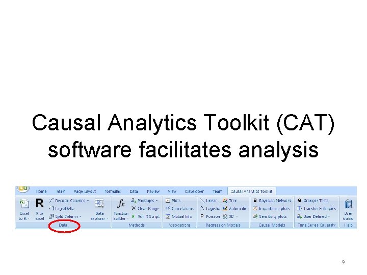
Causal Analytics Toolkit (CAT) software facilitates analysis 9

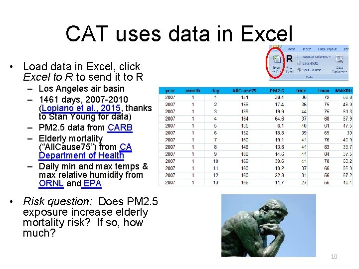
CAT uses data in Excel • Load data in Excel, click Excel to R to send it to R – Los Angeles air basin – 1461 days, 2007 -2010 (Lopiano et al. , 2015, thanks to Stan Young for data) – PM 2. 5 data from CARB – Elderly mortality (“All. Cause 75”) from CA Department of Health – Daily min and max temps & max relative humidity from ORNL and EPA • Risk question: Does PM 2. 5 exposure increase elderly mortality risk? If so, how much? 10

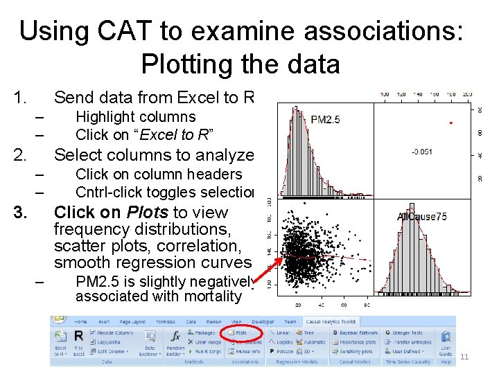
Using CAT to examine associations: Plotting the data 1. Send data from Excel to R – – 2. Highlight columns Click on “Excel to R” Select columns to analyze – – 3. Click on column headers Cntrl-click toggles selection Click on Plots to view frequency distributions, scatter plots, correlation, smooth regression curves – PM 2. 5 is slightly negatively associated with mortality 11

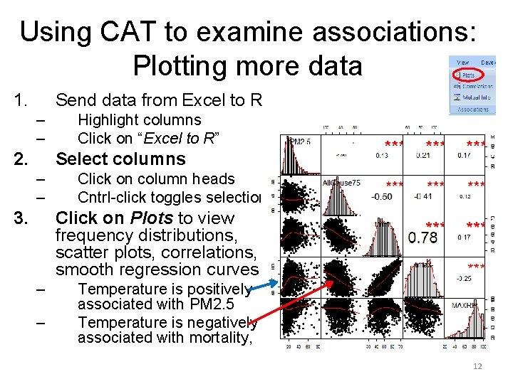
Using CAT to examine associations: Plotting more data 1. Send data from Excel to R – – 2. Highlight columns Click on “Excel to R” Select columns – – 3. Click on column heads Cntrl-click toggles selection Click on Plots to view frequency distributions, scatter plots, correlations, smooth regression curves – – Temperature is positively associated with PM 2. 5 Temperature is negatively associated with mortality, 12

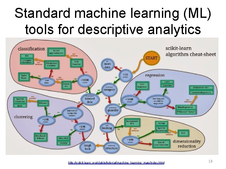
Standard machine learning (ML) tools for descriptive analytics http: //scikit-learn. org/stable/tutorial/machine_learning_map/index. html 13

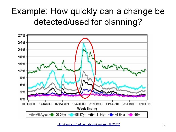
Example: How quickly can a change be detected/used for planning? http: //jamia. oxfordjournals. org/content/19/6/1075 14

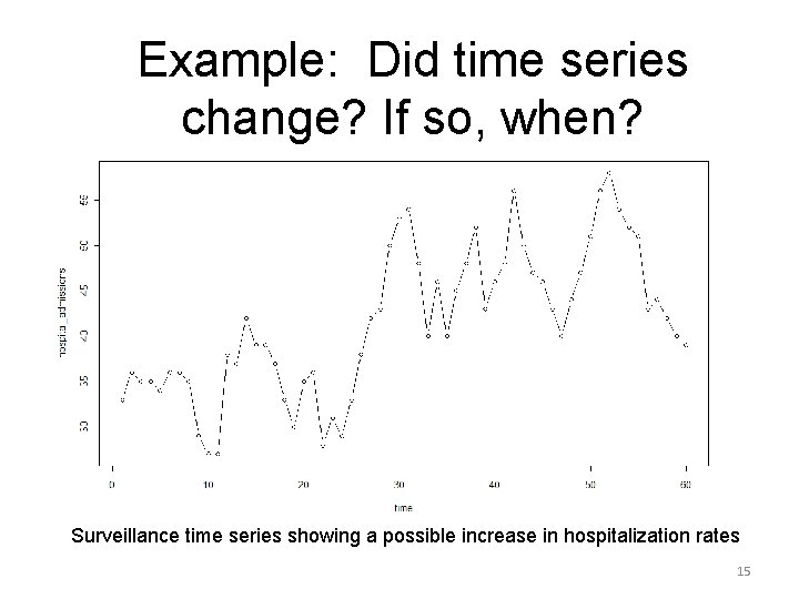
Example: Did time series change? If so, when? Surveillance time series showing a possible increase in hospitalization rates 15

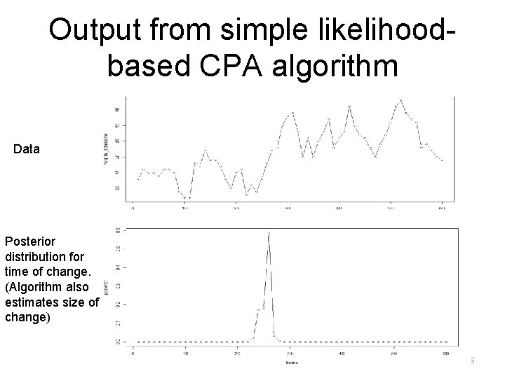
Output from simple likelihoodbased CPA algorithm Data Posterior distribution for time of change. (Algorithm also estimates size of change) 16

Algorithms for finding what has changed • Change-point analysis (CPA) – Basic idea: Search for most likely explanation of observed data – Provides estimates of • Times of changes • Sizes of changes • Confidence intervals and levels provided • Recent breakthroughs in CPA algorithms – Model-free CPA using order statistics – Multiple time series 17

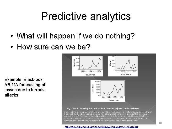
Predictive analytics • What will happen if we do nothing? • How sure can we be? Example: Black-box ARIMA forecasting of losses due to terrorist attacks 18 http: //www. slideshare. net/Victor. Odutokun/arima-analysis-project-slide

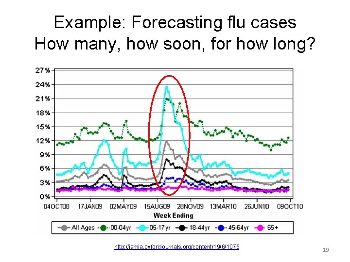
Example: Forecasting flu cases How many, how soon, for how long? http: //jamia. oxfordjournals. org/content/19/6/1075 19

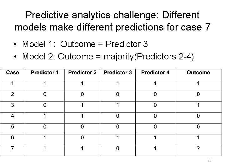
Predictive analytics challenge: Different models make different predictions for case 7 • Model 1: Outcome = Predictor 3 • Model 2: Outcome = majority(Predictors 2 -4) 20

Predictive analytics techniques • • Forecasting: Pr(future outputs | past) Regression: Pr(output | covariates) Dynamic simulation: Pr( outputs | inputs) Bayesian networks (BNs): Joint PDF – Inference: Pr(outputs | observed inputs) • Monte-Carlo and exact inference algorithms • Structure learning and ensemble learning algs – Dynamic Bayesian Networks (DBNs) • Kalman filtering and extensions • Particle swarm optimization 21

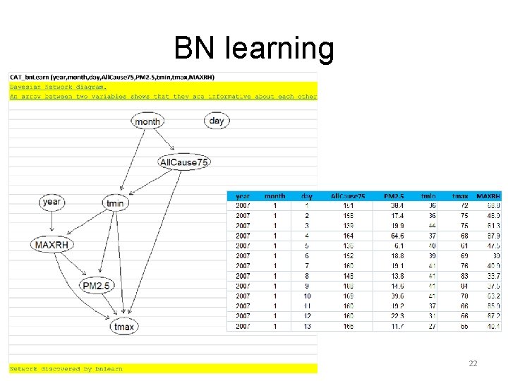
BN learning 22

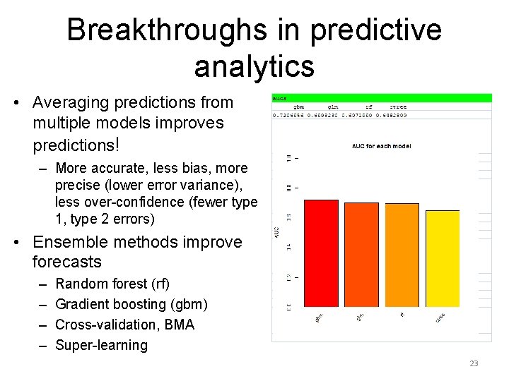
Breakthroughs in predictive analytics • Averaging predictions from multiple models improves predictions! – More accurate, less bias, more precise (lower error variance), less over-confidence (fewer type 1, type 2 errors) • Ensemble methods improve forecasts – – Random forest (rf) Gradient boosting (gbm) Cross-validation, BMA Super-learning 23

Causal analytics • Causal model: – Pr(outputs | input actions) – Pr(c | x) • Not BN inference, Pr(output | input observations) • How will future consequence probabilities change if we make different choices? • How do actions affect probable outcomes? 24

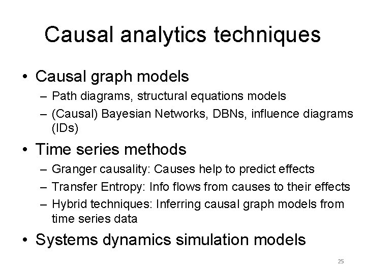
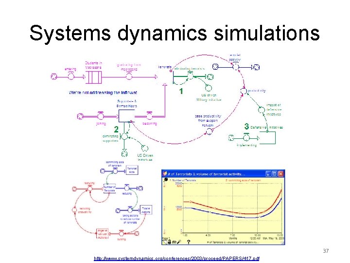
Causal analytics techniques • Causal graph models – Path diagrams, structural equations models – (Causal) Bayesian Networks, DBNs, influence diagrams (IDs) • Time series methods – Granger causality: Causes help to predict effects – Transfer Entropy: Info flows from causes to their effects – Hybrid techniques: Inferring causal graph models from time series data • Systems dynamics simulation models 25

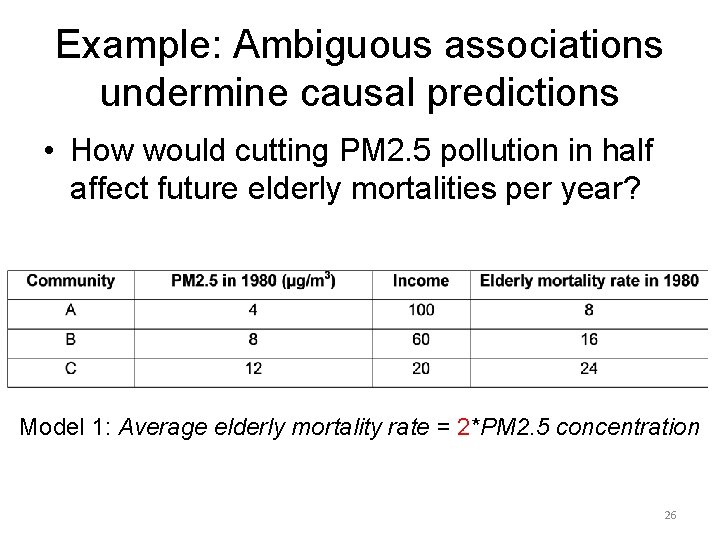
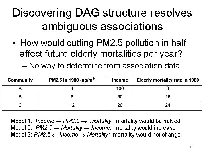
Example: Ambiguous associations undermine causal predictions • How would cutting PM 2. 5 pollution in half affect future elderly mortalities per year? Model 1: Average elderly mortality rate = 2*PM 2. 5 concentration 26

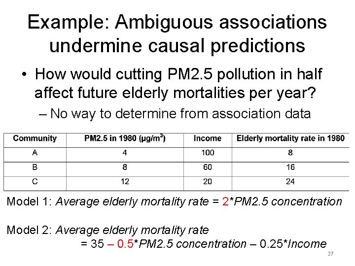
Example: Ambiguous associations undermine causal predictions • How would cutting PM 2. 5 pollution in half affect future elderly mortalities per year? – No way to determine from association data Model 1: Average elderly mortality rate = 2*PM 2. 5 concentration Model 2: Average elderly mortality rate = 35 – 0. 5*PM 2. 5 concentration – 0. 25*Income 27

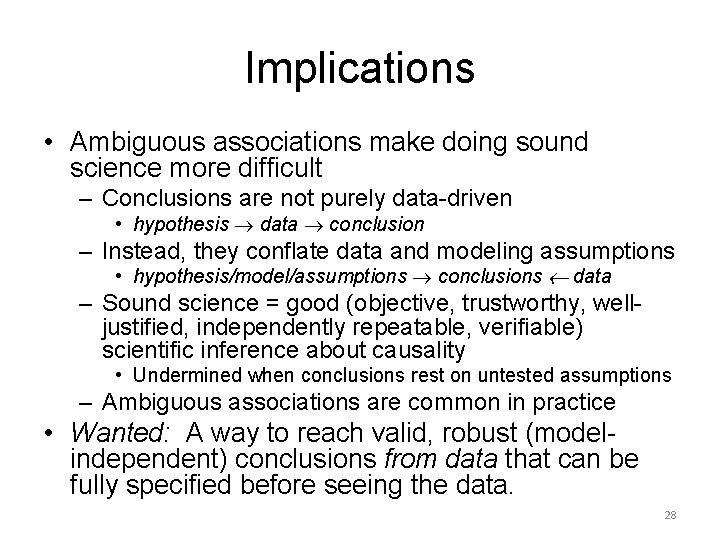
Implications • Ambiguous associations make doing sound science more difficult – Conclusions are not purely data-driven • hypothesis data conclusion – Instead, they conflate data and modeling assumptions • hypothesis/model/assumptions conclusions data – Sound science = good (objective, trustworthy, welljustified, independently repeatable, verifiable) scientific inference about causality • Undermined when conclusions rest on untested assumptions – Ambiguous associations are common in practice • Wanted: A way to reach valid, robust (modelindependent) conclusions from data that can be fully specified before seeing the data. 28

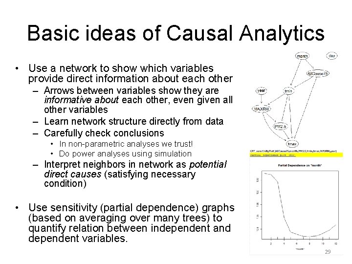
Basic ideas of Causal Analytics • Use a network to show which variables provide direct information about each other – Arrows between variables show they are informative about each other, even given all other variables – Learn network structure directly from data – Carefully check conclusions • In non-parametric analyses we trust! • Do power analyses using simulation – Interpret neighbors in network as potential direct causes (satisfying necessary condition) • Use sensitivity (partial dependence) graphs (based on averaging over many trees) to quantify relation between independent and dependent variables. 29

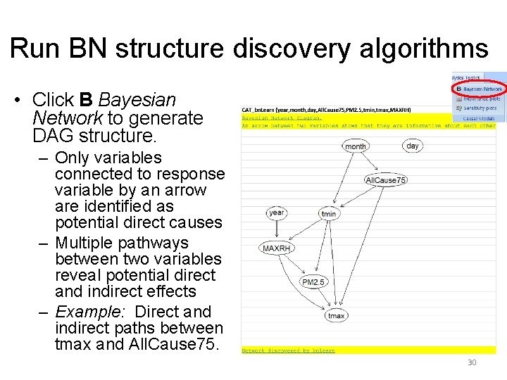
Run BN structure discovery algorithms • Click B Bayesian Network to generate DAG structure. – Only variables connected to response variable by an arrow are identified as potential direct causes – Multiple pathways between two variables reveal potential direct and indirect effects – Example: Direct and indirect paths between tmax and All. Cause 75. 30

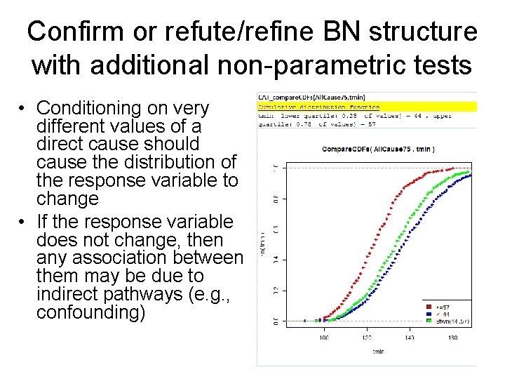
Confirm or refute/refine BN structure with additional non-parametric tests • Conditioning on very different values of a direct cause should cause the distribution of the response variable to change • If the response variable does not change, then any association between them may be due to indirect pathways (e. g. , confounding) 31

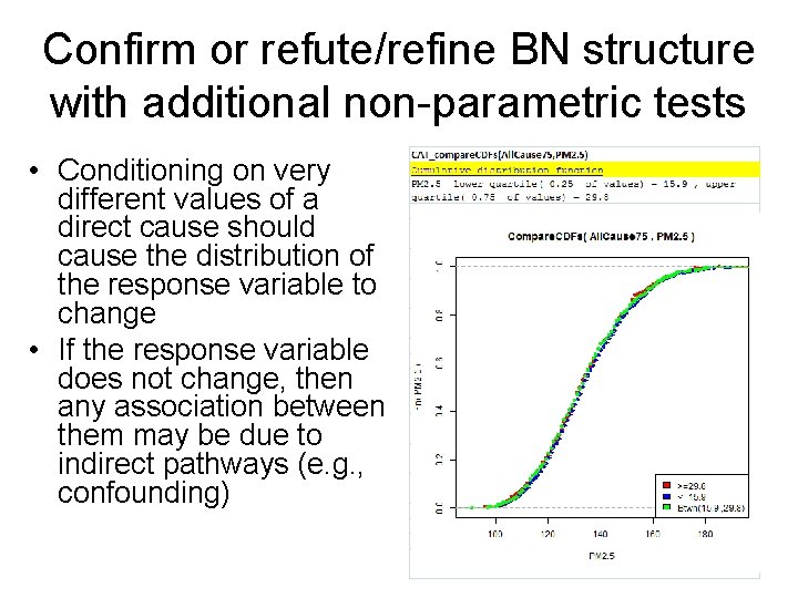
Confirm or refute/refine BN structure with additional non-parametric tests • Conditioning on very different values of a direct cause should cause the distribution of the response variable to change • If the response variable does not change, then any association between them may be due to indirect pathways (e. g. , confounding) 32

Discovering DAG structure resolves ambiguous associations • How would cutting PM 2. 5 pollution in half affect future elderly mortalities per year? – No way to determine from association data Model 1: Income PM 2. 5 Mortality: mortality would be halved Model 2: PM 2. 5 Mortality Income: mortality would increase Model 3: PM 2. 5 Income Mortality: mortality would not change 33

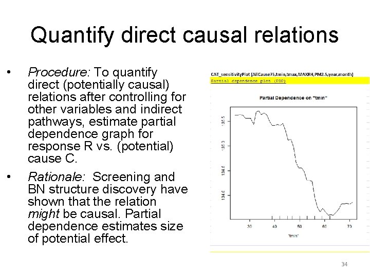
Quantify direct causal relations • • Procedure: To quantify direct (potentially causal) relations after controlling for other variables and indirect pathways, estimate partial dependence graph for response R vs. (potential) cause C. Rationale: Screening and BN structure discovery have shown that the relation might be causal. Partial dependence estimates size of potential effect. 34

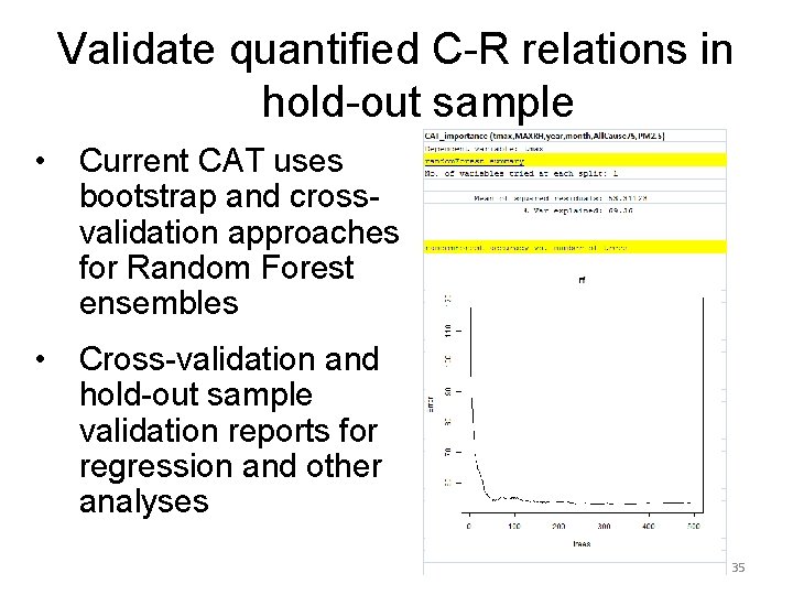
Validate quantified C-R relations in hold-out sample • Current CAT uses bootstrap and crossvalidation approaches for Random Forest ensembles • Cross-validation and hold-out sample validation reports for regression and other analyses 35

Summary of CAT’s causal analytics • Screen for total, partial, and temporal associations and information relations • Learn BN network structure from data • Estimate quantitative dependence relations among neighboring variables – Use partial dependence plots (Random Forest ensemble of non-parametric trees) – Use trees to quantify multivariate dependencies on multiple neighbors simultaneously • Validate on hold-out samples 36

Systems dynamics simulations 37 http: //www. systemdynamics. org/conferences/2003/proceed/PAPERS/417. pdf

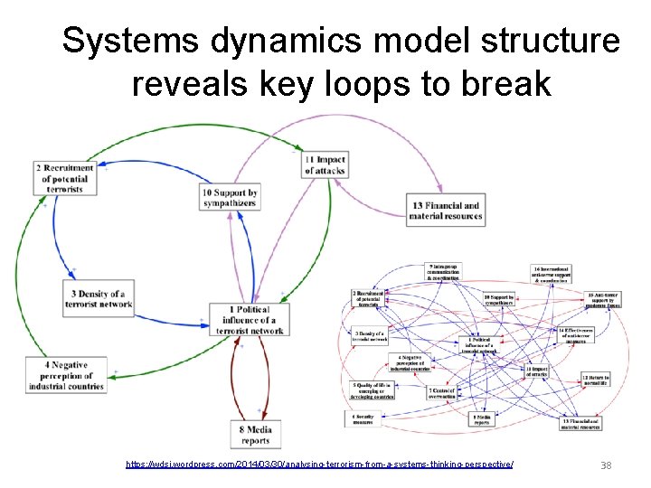
Systems dynamics model structure reveals key loops to break https: //wdsi. wordpress. com/2014/03/30/analysing-terrorism-from-a-systems-thinking-perspective/ 38

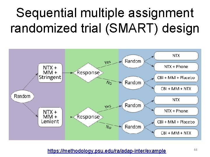
Prescriptive analytics • What to do next? – Uncertain models for predicting probable effects of different actions – Value-of-information – Exploration-exploitation trade-off • SMART trial design – Sequential multiple assignment randomized trials 39

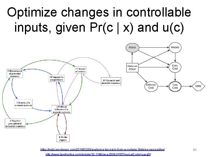
Optimize changes in controllable inputs, given Pr(c | x) and u(c) https: //wdsi. wordpress. com/2014/03/30/analysing-terrorism-from-a-systems-thinking-perspective/ http: //www. tandfonline. com/doi/abs/10. 1198/jasa. 2009. 0155? journal. Code=uasa 20 40

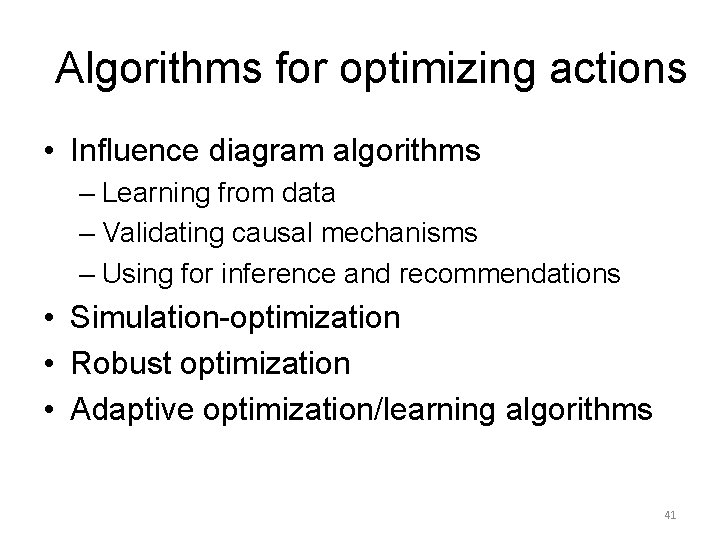
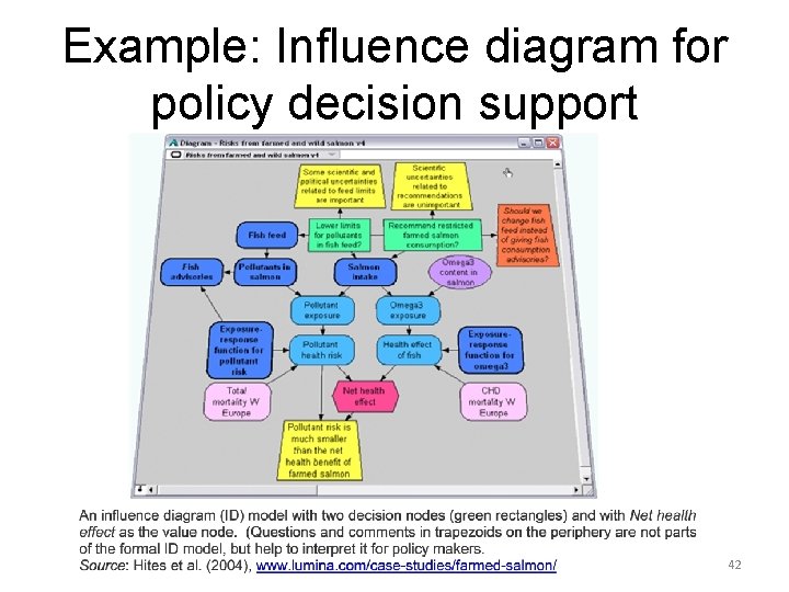
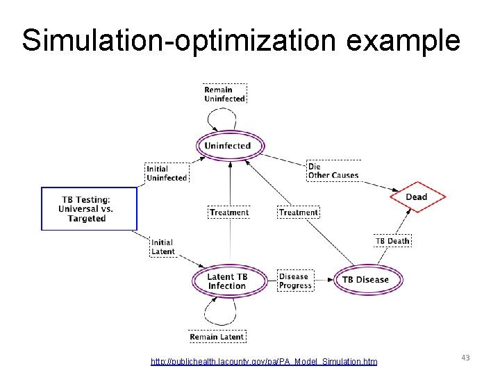
Algorithms for optimizing actions • Influence diagram algorithms – Learning from data – Validating causal mechanisms – Using for inference and recommendations • Simulation-optimization • Robust optimization • Adaptive optimization/learning algorithms 41

Example: Influence diagram for policy decision support 42

Simulation-optimization example http: //publichealth. lacounty. gov/pa/PA_Model_Simulation. htm 43

Sequential multiple assignment randomized trial (SMART) design https: //methodology. psu. edu/ra/adap-inter/example 44

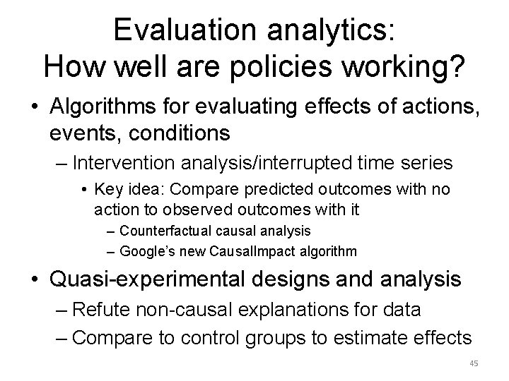
Evaluation analytics: How well are policies working? • Algorithms for evaluating effects of actions, events, conditions – Intervention analysis/interrupted time series • Key idea: Compare predicted outcomes with no action to observed outcomes with it – Counterfactual causal analysis – Google’s new Causal. Impact algorithm • Quasi-experimental designs and analysis – Refute non-causal explanations for data – Compare to control groups to estimate effects 45

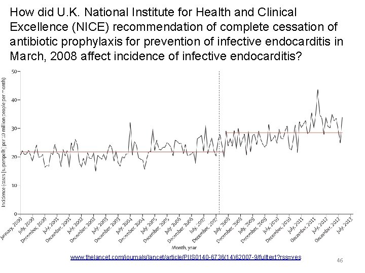
How did U. K. National Institute for Health and Clinical Excellence (NICE) recommendation of complete cessation of antibiotic prophylaxis for prevention of infective endocarditis in March, 2008 affect incidence of infective endocarditis? www. thelancet. com/journals/lancet/article/PIIS 0140 -6736(14)62007 -9/fulltext? rss=yes 46

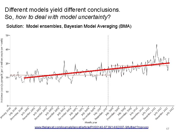
Different models yield different conclusions. So, how to deal with model uncertainty? Solution: Model ensembles, Bayesian Model Averaging (BMA) www. thelancet. com/journals/lancet/article/PIIS 0140 -6736(14)62007 -9/fulltext? rss=yes 47

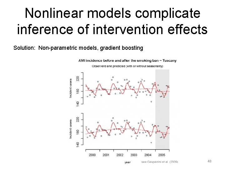
Nonlinear models complicate inference of intervention effects Solution: Non-parametric models, gradient boosting 48

Algorithms for evaluating effects of combinations of factors • Classification trees – Boosted trees, Random Forest, MARS • Bayesian Network algorithms – Discovery • Conditional independence tests – Validation – Inference and explanation • Response surface algorithms – Adaptive learning, design of experiments 49

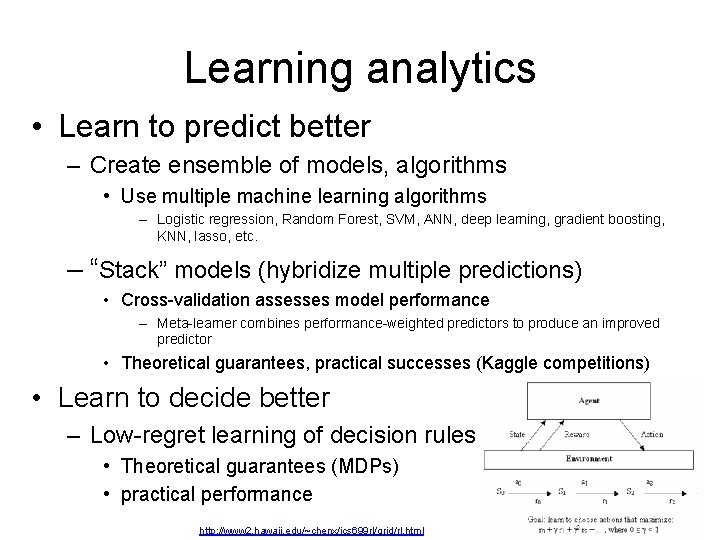
Learning analytics • Learn to predict better – Create ensemble of models, algorithms • Use multiple machine learning algorithms – Logistic regression, Random Forest, SVM, ANN, deep learning, gradient boosting, KNN, lasso, etc. – “Stack” models (hybridize multiple predictions) • Cross-validation assesses model performance – Meta-learner combines performance-weighted predictors to produce an improved predictor • Theoretical guarantees, practical successes (Kaggle competitions) • Learn to decide better – Low-regret learning of decision rules • Theoretical guarantees (MDPs) • practical performance 50 http: //www 2. hawaii. edu/~chenx/ics 699 rl/grid/rl. html

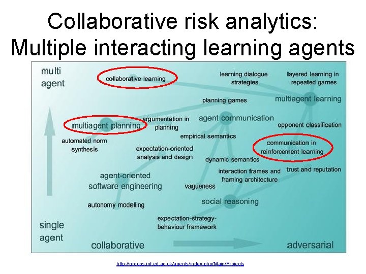
Collaborative risk analytics: Multiple interacting learning agents http: //groups. inf. ed. ac. uk/agents/index. php/Main/Projects 51

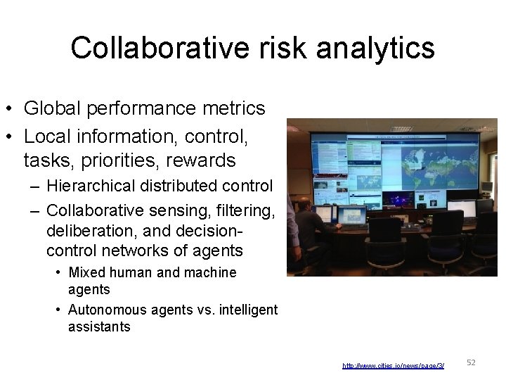
Collaborative risk analytics • Global performance metrics • Local information, control, tasks, priorities, rewards – Hierarchical distributed control – Collaborative sensing, filtering, deliberation, and decisioncontrol networks of agents • Mixed human and machine agents • Autonomous agents vs. intelligent assistants http: //www. cities. io/news/page/3/ 52

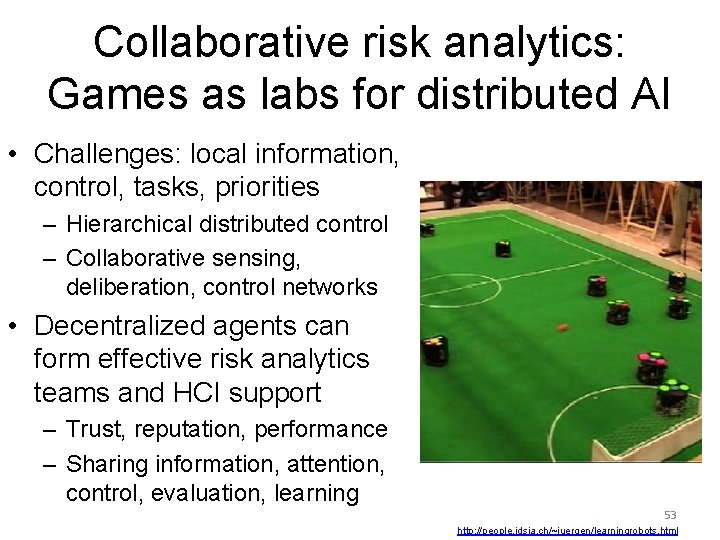
Collaborative risk analytics: Games as labs for distributed AI • Challenges: local information, control, tasks, priorities – Hierarchical distributed control – Collaborative sensing, deliberation, control networks • Decentralized agents can form effective risk analytics teams and HCI support – Trust, reputation, performance – Sharing information, attention, control, evaluation, learning 53 http: //people. idsia. ch/~juergen/learningrobots. html

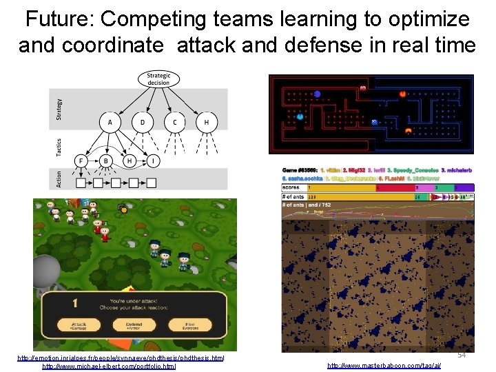
Future: Competing teams learning to optimize and coordinate attack and defense in real time http: //emotion. inrialpes. fr/people/synnaeve/phdthesis. html http: //www. michael-elbert. com/portfolio. html 54 http: //www. masterbaboon. com/tag/ai/

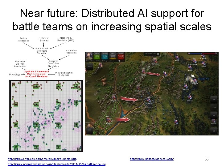
Near future: Distributed AI support for battle teams on increasing spatial scales http: //www 3. ntu. edu. sg/home/aswtcai/projects. htm http: //www. nowwithvitaminr. com/files/uploads/2011/05/daibattlecode. jpg http: //www. ultimategeneral. com/ 55

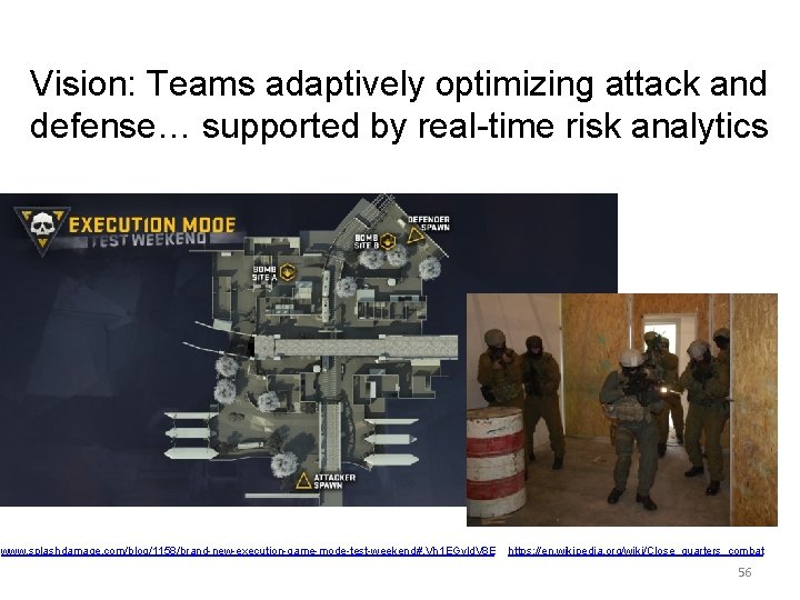
Vision: Teams adaptively optimizing attack and defense… supported by real-time risk analytics www. splashdamage. com/blog/1158/brand-new-execution-game-mode-test-weekend#. Vh 1 EGvld. V 8 E https: //en. wikipedia. org/wiki/Close_quarters_combat 56

Future: Trust autonomous agents for key tasks, such as sensing and responding to changes, seeking targets http: //www. gamasutra. com/view/feature/2484/using_particle_s warm_optimization_. php? print=1 http: //www. web. me. iastate. edu/sbhattac/group/pso. htm https: //www. reddit. com/r/starcitizen/comments/34 excc/looking_at_missile_me chanics_and_locking/ 57

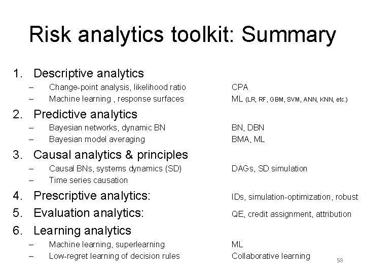
Risk analytics toolkit: Summary 1. Descriptive analytics – – Change-point analysis, likelihood ratio Machine learning , response surfaces CPA ML (LR, RF, GBM, SVM, ANN, KNN, etc. ) 2. Predictive analytics – – Bayesian networks, dynamic BN Bayesian model averaging BN, DBN BMA, ML 3. Causal analytics & principles – – Causal BNs, systems dynamics (SD) Time series causation 4. Prescriptive analytics: 5. Evaluation analytics: 6. Learning analytics – – Machine learning, superlearning Low-regret learning of decision rules DAGs, SD simulation IDs, simulation-optimization, robust QE, credit assignment, attribution ML Collaborative learning 58

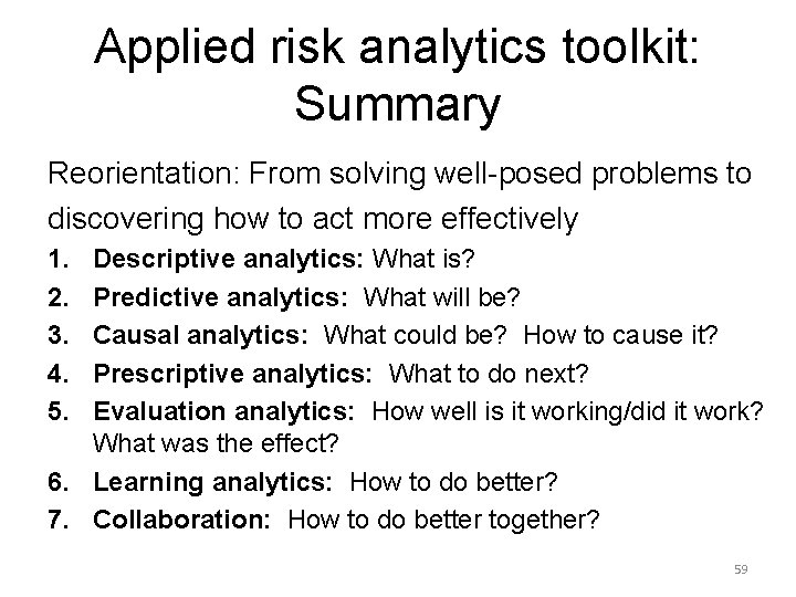
Applied risk analytics toolkit: Summary Reorientation: From solving well-posed problems to discovering how to act more effectively 1. 2. 3. 4. 5. Descriptive analytics: What is? Predictive analytics: What will be? Causal analytics: What could be? How to cause it? Prescriptive analytics: What to do next? Evaluation analytics: How well is it working/did it work? What was the effect? 6. Learning analytics: How to do better? 7. Collaboration: How to do better together? 59

Thanks! Questions? 60