Applied Quantitative Methods Lecture 7 Multiple Regression Analysis

Applied Quantitative Methods Lecture 7. Multiple Regression Analysis November 10 th, 2010

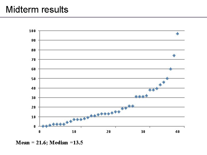
Midterm results 100 90 80 70 60 50 40 30 20 10 0 0 10 Mean = 21. 6; Median =13. 5 20 30 40

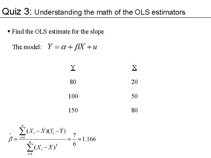
Quiz 3: Understanding the math of the OLS estimators § Find the OLS estimate for the slope The model: Y X 80 20 100 50 150 80

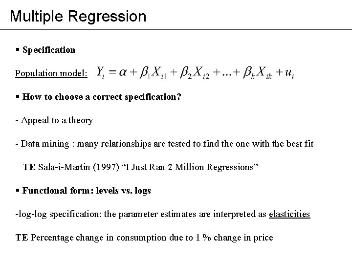
Multiple Regression § Specification Population model: § How to choose a correct specification? - Appeal to a theory - Data mining : many relationships are tested to find the one with the best fit TE Sala-i-Martin (1997) “I Just Ran 2 Million Regressions” § Functional form: levels vs. logs -log specification: the parameter estimates are interpreted as elasticities TE Percentage change in consumption due to 1 % change in price

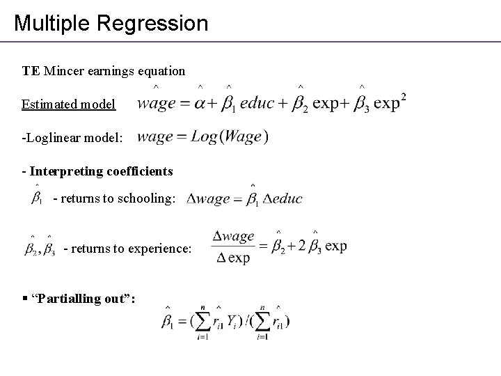
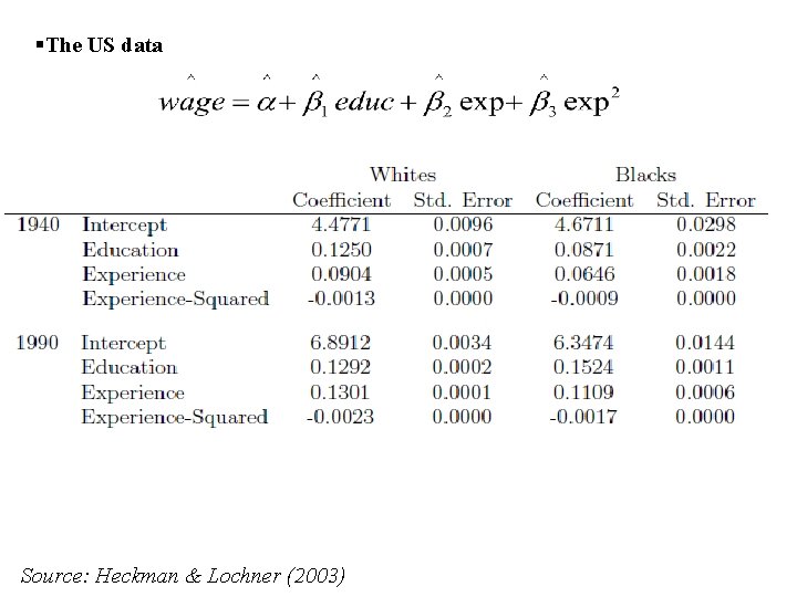
Multiple Regression TE Mincer earnings equation Estimated model -Loglinear model: - Interpreting coefficients - returns to schooling: - returns to experience: § “Partialling out”:

§The US data Source: Heckman & Lochner (2003)

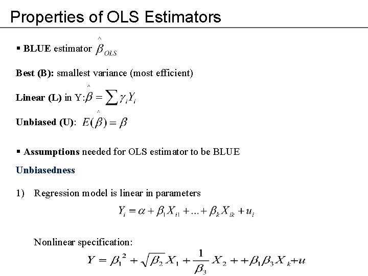
Properties of OLS Estimators § BLUE estimator Best (B): smallest variance (most efficient) Linear (L) in Y: Unbiased (U): § Assumptions needed for OLS estimator to be BLUE Unbiasedness 1) Regression model is linear in parameters Nonlinear specification:

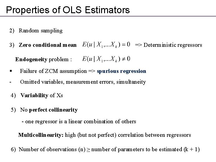
Properties of OLS Estimators 2) Random sampling 3) Zero conditional mean => Deterministic regressors Endogeneity problem : § Failure of ZCM assumption => spurious regression - Omitted variables, measurement errors, simultaneity 4) Variability of Xs 5) No perfect collinearity - one regressor is a linear combination of others Multicollinearity: high (but not perfect) correlation between regressors 6) Number of observations (n) ≥ number of parameters to be estimated (k + 1)

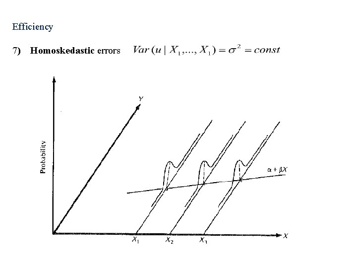
Efficiency 7) Homoskedastic errors

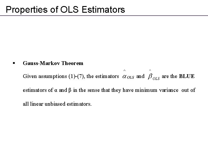
Properties of OLS Estimators § Gauss-Markov Theorem Given assumptions (1)-(7), the estimators and are the BLUE estimators of α and β in the sense that they have minimum variance out of all linear unbiased estimators.

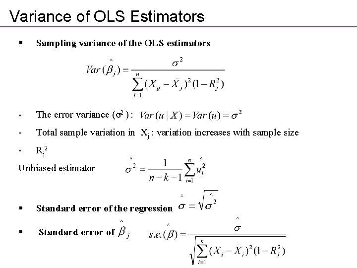
Variance of OLS Estimators § Sampling variance of the OLS estimators - The error variance (σ2 ) : - Total sample variation in Xj : variation increases with sample size - Rj 2 Unbiased estimator § Standard error of the regression § Standard error of

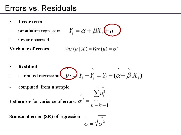
Errors vs. Residuals § Error term - population regression - never observed Variance of errors § Residual - estimated regression - computed from a sample Estimator for variance of errors: Standard error (SE) of regression

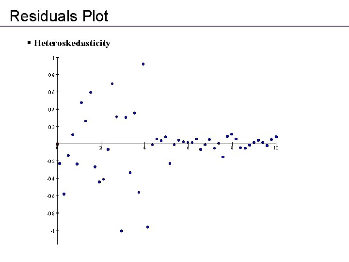
Residuals Plot § Heteroskedasticity

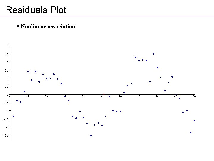
Residuals Plot § Nonlinear association

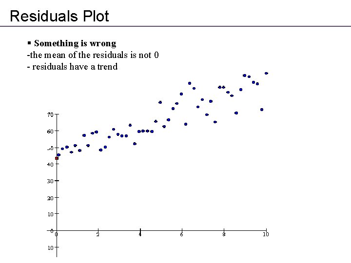
Residuals Plot § Something is wrong -the mean of the residuals is not 0 - residuals have a trend

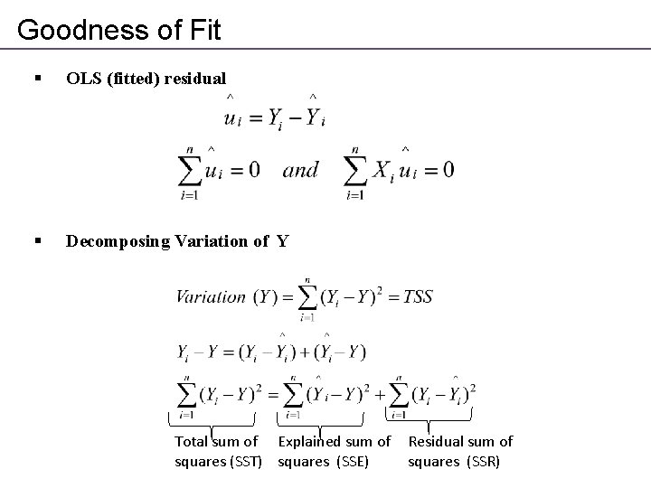
Goodness of Fit § OLS (fitted) residual § Decomposing Variation of Y Total sum of Explained sum of squares (SST) squares (SSE) Residual sum of squares (SSR)

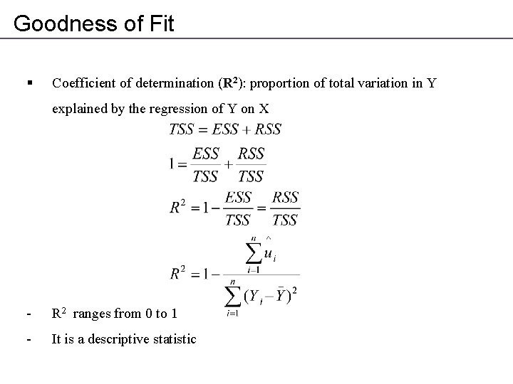
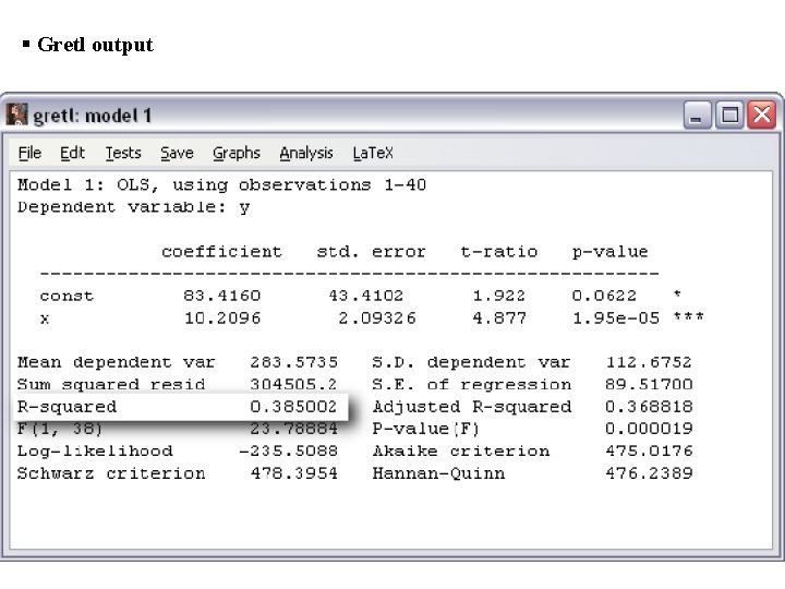
Goodness of Fit § Coefficient of determination (R 2): proportion of total variation in Y explained by the regression of Y on X - R 2 ranges from 0 to 1 - It is a descriptive statistic

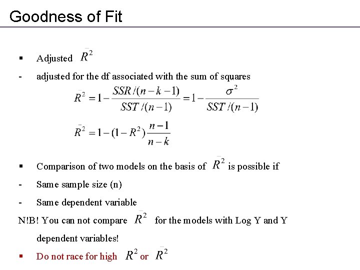
Goodness of Fit § Adjusted - adjusted for the df associated with the sum of squares § Comparison of two models on the basis of - Same sample size (n) - Same dependent variable N!B! You can not compare for the models with Log Y and Y dependent variables! § Do not race for high is possible if or

§ Gretl output

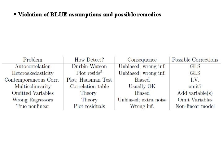
§ Violation of BLUE assumptions and possible remedies

Next Lecture Multiple Regression Analysis: Inferences ! Wooldridge, Chapter 4 & 6 Paper: Barro & Mc. Cleary. Religion and Economic Growth. NBER Working Paper 9682, May 2003