Applied Quantitative Analysis and Practices LECTURE32 By Dr

Applied Quantitative Analysis and Practices LECTURE#32 By Dr. Osman Sadiq Paracha

Defining and Collecting Data
 variables have values that can only be")
Types of Variables § § Categorical (qualitative) variables have values that can only be placed into categories, such as “yes” and “no. ” Numerical (quantitative) variables have values that represent a counted or measured quantity. § § Discrete variables arise from a counting process Continuous variables arise from a measuring process

Types of Variables Categorical Numerical Examples: n n n Marital Status Political Party Eye Color (Defined categories) Discrete Examples: n n Number of Children Defects per hour (Counted items) Continuous Examples: n n Weight Voltage (Measured characteristics)

Levels of Measurement A nominal scale classifies data into distinct categories in which no ranking is implied. Categorical Variables Categories Do you have a Facebook profile? Yes, No Type of investment Growth , Value, Other Cellular Provider AT&T, Sprint, Verizon, Other, None
 An ordinal scale classifies data into distinct categories in")
Levels of Measurement (con’t. ) An ordinal scale classifies data into distinct categories in which ranking is implied Categorical Variable Ordered Categories Student class designation Freshman, Sophomore, Junior, Senior Product satisfaction Very unsatisfied, Fairly unsatisfied, Neutral, Fairly satisfied, Very satisfied Faculty rank Professor, Associate Professor, Assistant Professor, Instructor Standard & Poor’s bond ratings AAA, A, BBB, B, CCC, C, DDD, D Student Grades A, B, C, D, F
 § § An interval scale is an ordered scale")
Levels of Measurement (con’t. ) § § An interval scale is an ordered scale in which the difference between measurements is a meaningful quantity but the measurements do not have a true zero point. A ratio scale is an ordered scale in which the difference between the measurements is a meaningful quantity and the measurements have a true zero point.

Sources of Data § Primary Sources: The data collector is the one using the data for analysis § Data from a political survey § Data collected from an experiment § Observed data § Secondary Sources: The person performing data analysis is not the data collector § Analyzing census data § Examining data from print journals or data published on the internet.

Population vs. Sample Population All the items or individuals about which you want to draw conclusion(s) Sample A portion of the population of items or individuals

Types of Samples Non-Probability Samples Judgment Convenience Probability Samples Simple Random Stratified Systematic Cluster

Evaluating Survey Worthiness n n n What is the purpose of the survey? Is the survey based on a probability sample? Coverage error – appropriate frame? Nonresponse error – follow up Measurement error – good questions elicit good responses Sampling error – always exists
 n Coverage error Excluded from frame n Nonresponse error")
Types of Survey Errors (continued) n Coverage error Excluded from frame n Nonresponse error Follow up on nonresponses n Sampling error Random differences from sample to sample n Measurement error Bad or leading question

Organizing and Visualizing Variables

Categorical Data Are Organized By Utilizing Tables Categorical Data Tallying Data One Categorical Variable Two Categorical Variables Summary Table Contingency Table

Contingency Table - Example n n A random sample of 400 Contingency Table Showing invoices is drawn. Frequency of Invoices Categorized Each invoice is categorized By Size and The Presence Of Errors as a small, medium, or large No Errors Total amount. Small 170 20 190 Each invoice is also Amount examined to identify if there Medium 100 40 140 are any errors. Amount This data are then organized Large 65 5 70 Amount in the contingency table to the right. 335 65 400 Total
 IN ABBOTTABAD (2000 -2011)")
PAST TRENDS IN SSC RESULTS IN GOVT HIGH SCHOOLS (FEMALE) IN ABBOTTABAD (2000 -2011) Comparison of No of Students Appeared with No of Students Passed (Female Govt High Schools)(2000 -2011) 3500 NUMBER OF STUDENTS 3000 2919 2689 2500 2478 2211 2000 1960 1766 1772 1500 1223 1000 1329 1897 2211 2176 1935 2113 1891 1481 1347 1375 1942 1451 500 0 2001 2002 2003 2004 2005 2006 YEAR 2007 2008 1832 No of Students Appeared No of Students Passed 1135 1118 2533 2009 2010 2011

Organizing Numerical Data: Frequency Distribution § § The frequency distribution is a summary table in which the data are arranged into numerically ordered classes. You must give attention to selecting the appropriate number of class groupings for the table, determining a suitable width of a class grouping, and establishing the boundaries of each class grouping to avoid overlapping. The number of classes depends on the number of values in the data. With a larger number of values, typically there are more classes. In general, a frequency distribution should have at least 5 but no more than 15 classes. To determine the width of a class interval, you divide the range (Highest value–Lowest value) of the data by the number of class groupings desired.

Visualizing Categorical Data Through Graphical Displays Categorical Data Visualizing Data Summary Table For One Variable Bar Chart Pie Chart Contingency Table For Two Variables Side By Side Bar Chart

Visualizing Numerical Data By Using Graphical Displays Numerical Data Ordered Array Stem-and-Leaf Display Frequency Distributions and Cumulative Distributions Histogram Polygon Ogive

Visualizing Numerical Data: The Histogram Class 10 but less than 20 20 but less than 30 30 but less than 40 40 but less than 50 50 but less than 60 Total Frequency 3 6 5 4 2 20 (In a percentage histogram the vertical axis would be defined to show the percentage of observations per class) Relative Frequency . 15. 30. 25. 20. 10 1. 00 Percentage 15 30 25 20 10 100

Visualizing Two Numerical Variables By Using Graphical Displays Two Numerical Variables Scatter Plot Time. Series Plot

Time Series Plot Example Year Number of Franchises 1996 43 1997 54 1998 60 1999 73 2000 82 2001 95 2002 107 2003 99 2004 95
 IN ABBOTTABAD (2000 -2011)")
PAST TRENDS IN SSC RESULTS IN GOVT HIGH SCHOOLS (FEMALE) IN ABBOTTABAD (2000 -2011) Comparison of No of Students Appeared with No of Students Passed (Female Govt High Schools)(2000 -2011) 3500 NUMBER OF STUDENTS 3000 2919 2689 2500 2478 2211 2000 1960 1766 1772 1500 1223 1000 1329 1897 2211 2176 1935 2113 1891 1481 1347 1375 1942 1451 500 0 2001 2002 2003 2004 2005 2006 YEAR 2007 2008 1832 No of Students Appeared No of Students Passed 1135 1118 2533 2009 2010 2011

Guidelines For Avoiding The Obscuring Of Data § § § § Avoid chartjunk Use the simplest possible visualization Include a title Label all axes Include a scale for each axis if the chart contains axes Begin the scale for a vertical axis at zero Use a constant scale

Numerical Descriptive Measures

Summary Definitions § § § The central tendency is the extent to which all the data values group around a typical or central value. The variation is the amount of dispersion or scattering of values The shape is the pattern of the distribution of values from the lowest value to the highest value.
 n n n The most common measure")
Measures of Central Tendency: The Mean (con’t) n n n The most common measure of central tendency Mean = sum of values divided by the number of values Affected by extreme values (outliers) 11 12 13 14 15 16 17 18 19 20 Mean = 13 11 12 13 14 15 16 17 18 19 20 Mean = 14

Measures of Central Tendency: The Median n In an ordered array, the median is the “middle” number (50% above, 50% below) 11 12 13 14 15 16 17 18 19 20 Median = 13 n Less sensitive than the mean to extreme values

Measures of Central Tendency: The Mode n n n Value that occurs most often Not affected by extreme values Used for either numerical or categorical (nominal) data There may be no mode There may be several modes 0 1 2 3 4 5 6 7 8 9 10 11 12 13 14 Mode = 9 0 1 2 3 4 5 6 No Mode

Measures of Central Tendency: Summary Central Tendency Arithmetic Mean Median Middle value in the ordered array Mode Most frequently observed value Geometric Mean Rate of change of a variable over time

Measures of Variation Range n Variance Measures of variation give information on the spread or variability or dispersion of the data values. Standard Deviation Coefficient of Variation Same center, different variation

Measures of Variation: The Range § § Simplest measure of variation Difference between the largest and the smallest values: Range = Xlargest – Xsmallest Example: 0 1 2 3 4 5 6 7 8 9 10 11 12 Range = 13 - 1 = 12 13 14

Measures of Variation: Why The Range Can Be Misleading § Does not account for how the data are distributed 7 8 9 10 11 12 7 8 Range = 12 - 7 = 5 § 9 10 11 Range = 12 - 7 = 5 Sensitive to outliers 1, 1, 1, 2, 2, 3, 3, 4, 5 Range = 5 - 1 = 4 1, 1, 1, 2, 2, 3, 3, 4, 120 Range = 120 - 1 = 119 12
 of squared deviations of values")
Measures of Variation: The Sample Variance n Average (approximately) of squared deviations of values from the mean n Sample variance: Where = arithmetic mean n = sample size Xi = ith value of the variable X

Measures of Variation: The Sample Standard Deviation n n Most commonly used measure of variation Shows variation about the mean Is the square root of the variance Has the same units as the original data n Sample standard deviation:

Measures of Variation: Comparing Standard Deviations Data A 11 12 13 14 15 16 17 18 19 20 21 Mean = 15. 5 S = 3. 338 20 Mean = 15. 5 S = 0. 926 Data B 11 21 12 13 14 15 16 17 18 19 Data C 11 12 13 14 15 16 17 18 19 20 21 Mean = 15. 5 S = 4. 567

Measures of Variation: Comparing Standard Deviations Smaller standard deviation Larger standard deviation

Locating Extreme Outliers: Z-Score § § To compute the Z-score of a data value, subtract the mean and divide by the standard deviation. The Z-score is the number of standard deviations a data value is from the mean. A data value is considered an extreme outlier if its Zscore is less than -3. 0 or greater than +3. 0. The larger the absolute value of the Z-score, the farther the data value is from the mean.
 n Measures the extent to which data is not")
Shape of a Distribution (Skewness) n Measures the extent to which data is not symmetrical Left-Skewed Symmetric Right-Skewed Mean < Median Mean = Median < Mean Skewness Statistic <0 0 >0

Quartile Measures n Quartiles split the ranked data into 4 segments with an equal number of values per segment 25% Q 1 n n n 25% Q 2 25% Q 3 The first quartile, Q 1, is the value for which 25% of the observations are smaller and 75% are larger Q 2 is the same as the median (50% of the observations are smaller and 50% are larger) Only 25% of the observations are greater than the third quartile
")
Calculating The Interquartile Range Example: X minimum Q 1 25% 12 Median (Q 2) 25% 30 25% 45 X Q 3 maximum 25% 57 Interquartile range = 57 – 30 = 27 70

Five Number Summary and The Boxplot n The Boxplot: A Graphical display of the data based on the five-number summary: Xsmallest -- Q 1 -- Median -- Q 3 -- Xlargest Example: 25% of data Xsmallest 25% of data Q 1 25% of data Median 25% of data Q 3 Xlargest

The Empirical Rule n n The empirical rule approximates the variation of data in a bell-shaped distribution Approximately 68% of the data in a bell shaped distribution is within 1 standard deviation of the mean or 68%

The Empirical Rule n n Approximately 95% of the data in a bell-shaped distribution lies within two standard deviations of the mean, or µ ± 2σ Approximately 99. 7% of the data in a bell-shaped distribution lies within three standard deviations of the mean, or µ ± 3σ 95% 99. 7%

The Covariance n The covariance measures the strength of the linear relationship between two numerical variables (X & Y) n The sample covariance: n Only concerned with the strength of the relationship n No causal effect is implied

Coefficient of Correlation n n Measures the relative strength of the linear relationship between two numerical variables Sample coefficient of correlation: where

Features of the Coefficient of Correlation n The population coefficient of correlation is referred as ρ. n The sample coefficient of correlation is referred to as r. n Either ρ or r have the following features: n Unit free n Range between – 1 and 1 n The closer to – 1, the stronger the negative linear relationship n The closer to 1, the stronger the positive linear relationship n The closer to 0, the weaker the linear relationship

Scatter Plots of Sample Data with Various Coefficients of Correlation Y Y r = -1 Y X r = -. 6 Y Y r = +1 X X r = +. 3 X r=0 X

SPSS Applications

Correlation and Causality n The third-variable problem: n n in any correlation, causality between two variables cannot be assumed because there may be other measured or unmeasured variables affecting the results. Direction of causality: n Correlation coefficients say nothing about which variable causes the other to change

Correlation n Spearman’s Rho n n Pearson’s correlation on the ranked data Kendall’s Tau n Better than Spearman’s for small samples

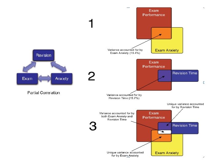
Partial Correlations n Partial correlation: n Measures the relationship between two variables, controlling for the effect that a third variable has on them both

The Normal Distribution

n n Discrete variables produce outcomes that come from a counting process (e. g. number of classes you are taking). Continuous variables produce outcomes that come from a measurement (e. g. your annual salary, or your weight).

Types Of Variables Discrete Variable Continuous Variable

The Normal Distribution ‘Bell Shaped’ n Symmetrical n Mean, Median and Mode are Equal Location is determined by the mean, μ n Spread is determined by the standard deviation, σ The random variable has an infinite theoretical range: + to f(X) σ μ Mean = Median = Mode X
 Changing μ shifts the distribution left or right. σ")
The Normal Distribution Shape f(X) Changing μ shifts the distribution left or right. σ μ Changing σ increases or decreases the spread. X

The Standardized Normal Distribution n Also known as the “Z” distribution Mean is 0 Standard Deviation is 1 f(Z) 1 0 Z Values above the mean have positive Z-values. Values below the mean have negative Z-values.
 P")
Finding Normal Probabilities Probability is measured by the area under the curve f(X) P (a ≤ X ≤ b) = P (a < X < b) (Note that the probability of any individual value is zero) a b X

Probability as Area Under the Curve The total area under the curve is 1. 0, and the curve is symmetric, so half is above the mean, half is below f(X) 0. 5 μ X

The Standardized Normal Table The Cumulative Standardized Normal table gives the probability less than a desired value of Z (i. e. , from negative infinity to Z) n 0. 9772 Example: P(Z < 2. 00) = 0. 9772 0 2. 00 Z
 The column gives the value of Z to the")
The Standardized Normal Table (continued) The column gives the value of Z to the second decimal point Z The row shows the value of Z to the first decimal point 0. 00 0. 01 0. 02 … 0. 0 0. 1 . . . 2. 0 P(Z < 2. 00) = 0. 9772 The value within the table gives the probability from Z = up to the desired Z value
 when")
General Procedure for Finding Normal Probabilities To find P(a < X < b) when X is distributed normally: n Draw the normal curve for the problem in terms of X n Translate X-values to Z-values n Use the Standardized Normal Table

Evaluating Normality n n n Not all continuous distributions are normal It is important to evaluate how well the data set is approximated by a normal distribution. Normally distributed data should approximate theoretical normal distribution: n n n The normal distribution is bell shaped (symmetrical) where the mean is equal to the median. The empirical rule applies to the normal distribution. The interquartile range of a normal distribution is 1. 33 standard deviations.
 Comparing data characteristics to theoretical properties n Construct charts or graphs")
Evaluating Normality (continued) Comparing data characteristics to theoretical properties n Construct charts or graphs n n n For small- or moderate-sized data sets, construct a stem-and-leaf display or a boxplot to check for symmetry For large data sets, does the histogram or polygon appear bellshaped? Compute descriptive summary measures n n n Do the mean, median and mode have similar values? Is the interquartile range approximately 1. 33σ? Is the range approximately 6σ?

Constructing A Normal Probability Plot n Normal probability plot n n Arrange data into ordered array Find corresponding standardized normal quantile values (Z) Plot the pairs of points with observed data values (X) on the vertical axis and the standardized normal quantile values (Z) on the horizontal axis Evaluate the plot for evidence of linearity

The Normal Probability Plot Interpretation A normal probability plot for data from a normal distribution will be approximately linear: X 90 60 30 -2 -1 0 1 2 Z

Building Statistical Models

Model Formulating Process

Generating and Testing Theories n n Hypothesis n n n An hypothesized general principle or set of principles that explain known findings about a topic and from which new hypotheses can be generated. A prediction from a theory. E. g. , Firms investing in their human resources will generate more profit. Falsification n The act of disproving a theory or hypothesis.

Collect Data to Test Your Theory n Hypothesis: n n Independent Variable n n Employee training improves employee productivity. The proposed cause A predictor variable Employee training in the hypothesis above Dependent Variable n n n The proposed effect An outcome variable Employee productivity in the hypothesis above
 about a")
What is a Hypothesis? n DCOVA A hypothesis is a claim (assertion) about a population parameter: n population mean Example: The mean monthly cell phone bill in this city is μ = $42 n population proportion Example: The proportion of adults in this city with cell phones is π = 0. 68

The Null Hypothesis, H 0 n DCOVA States the claim or assertion to be tested Example: The mean diameter of a manufactured bolt is 30 mm ( ) n Is always about a population parameter, not about a sample statistic
 n n Begin with the assumption that")
The Null Hypothesis, H 0 DCOVA (continued) n n Begin with the assumption that the null hypothesis is true n Similar to the notion of innocent until proven guilty Refers to the status quo or historical value Always contains “=“, or “≤”, or “≥” sign May or may not be rejected

The Alternative Hypothesis, H 1 DCOVA n Is the opposite of the null hypothesis n n n e. g. , The average diameter of a manufactured bolt is not equal to 30 mm ( H 1: μ ≠ 30 ) Challenges the status quo Never contains the “=“, or “≤”, or “≥” sign May or may not be proven Is generally the hypothesis that the researcher is trying to prove

The Test Statistic and Critical Values DCOVA n n If the sample mean is close to the stated population mean, the null hypothesis is not rejected. If the sample mean is far from the stated population mean, the null hypothesis is rejected. How far is “far enough” to reject H 0? The critical value of a test statistic creates a “line in the sand” for decision making -- it answers the question of how far is far enough.

The Test Statistic and Critical Values DCOVA Sampling Distribution of the test statistic Region of Rejection Region of Non-Rejection Region of Rejection Critical Values “Too Far Away” From Mean of Sampling Distribution
 Possible Hypothesis Test Outcomes Actual")
Possible Errors in Hypothesis Test DCOVA Decision Making (continued) Possible Hypothesis Test Outcomes Actual Situation Decision H 0 True H 0 False Do Not Reject H 0 No Error Probability 1 - α Type II Error Probability β Reject H 0 Type I Error Probability α No Error Power 1 - β
 n n n The confidence")
Possible Errors in Hypothesis Test DCOVA Decision Making (continued) n n n The confidence coefficient (1 -α) is the probability of not rejecting H 0 when it is true. The confidence level of a hypothesis test is α)*100%. The power of a statistical test (1 -β) is the probability of rejecting H 0 when it is false. (1 -

Type I & II Error Relationship DCOVA § Type I and Type II errors cannot happen at the same time § A Type I error can only occur if H 0 is true § A Type II error can only occur if H 0 is false If Type I error probability ( ) Type II error probability (β) , then

Factors Affecting Type II Error DCOVA n All else equal, n β when the difference between hypothesized parameter and its true value n β when σ n β when n

Level of Significance and the Rejection Region H 0: μ = 30 H 1: μ ≠ 30 DCOVA Level of significance = a a /2 30 Critical values Rejection Region This is a two-tail test because there is a rejection region in both tails

p-Value Approach to Testing DCOVA n p-value: Probability of obtaining a test statistic equal to or more extreme than the observed sample value given H 0 is true n n The p-value is also called the observed level of significance It is the smallest value of for which H 0 can be rejected
 Unknown (t test)")
Hypothesis Tests for the Mean Hypothesis Tests for Known (Z test) Unknown (t test)

Assumptions for normal distribution n Tests based on the normal distribution assume: n n Additivity and linearity Normality Homogeneity of Variance Independence

Reducing Bias n Trim the data: n n Windsorizing: n n Substitute outliers with the highest value that isn’t an outlier Analyse with Robust Methods: n n Delete a certain amount of scores from the extremes. Bootstrapping Transform the data: n By applying a mathematical function to scores.
) n n Square Root Transformation (√Xi): n n")
Transforming Data n Log Transformation (log(Xi)) n n Square Root Transformation (√Xi): n n Reduce positive skew. Also reduces positive skew. Can also be useful for stabilizing variance. Reciprocal Transformation (1/ Xi): n Dividing 1 by each score also reduces the impact of large scores. This transformation reverses the scores, you can avoid this by reversing the scores before the transformation, 1/(XHighest – Xi).

Log Transformation Before After

Square Root Transformation Before After

Reciprocal Transformation Before After

But … Before After

To Transform … Or Not n n Transforming the data helps as often as it hinders the accuracy of F. According to researchers: n The central limit theorem: sampling distribution will be normal in samples > 40 anyway. n Transforming the data changes the hypothesis being tested n E. g. when using a log transformation and comparing means you change from comparing arithmetic means to comparing geometric means n In small samples it is tricky to determine normality one way or another. n The consequences for the statistical model of applying the ‘wrong’ transformation could be worse than the consequences of analysing the untransformed scores.

Reliability n n The ability of the measure to produce the same results under the same conditions. Test-Retest Reliability n The ability of a measure to produce consistent results when the same entities are tested at two different points in time.

Cronbach’s alpha assessing scale reliability

Cronbach’s alpha } } Cronbach's alpha is an index of reliability associated with the variation accounted for by the true score of the "underlying construct. " Allows a researcher to measure the internal consistency of scale items, based on the average inter -item correlation Indicates the extent to which the items in your questionnaire are related to each other Indicates whether a scale is unidimensional or multidimensional

Interpreting scale reliability } } The higher the score, the more reliable the generated scale is A score of. 70 or greater is generally considered to be acceptable n n } . 90 or > = high reliability. 80 -. 89 = good reliability. 70 -79 = acceptable reliability. 65 -. 69 = marginal reliability lower thresholds are sometimes used in the literature.

Validity n n Whether an instrument measures what it set out to measure. Content validity n n Evidence that the content of a test corresponds to the content of the construct it was designed to cover Construct validity n Construct validity involves adoption of complex statistical methods to validate the constructs making it preferable over other types of validity.

Exploratory Factor Analysis

Exploratory Factor Analysis Defined Exploratory factor analysis. . . is an interdependence technique whose primary purpose is to define the underlying structure among the variables in the analysis.

What is Exploratory Factor Analysis? Exploratory Factor Analysis. . . • • • Examines the interrelationships among a large number of variables and then attempts to explain them in terms of their common underlying dimensions. These common underlying dimensions are referred to as factors. A summarization and data reduction technique that does not have independent and dependent variables, but is an interdependence technique in which all variables are considered simultaneously.
 = is used to discover")
Types of Factor Analysis 1. Exploratory Factor Analysis (EFA) = is used to discover the factor structure of a construct and examine its reliability. It is data driven. 2. Confirmatory Factor Analysis (CFA) = is used to confirm the fit of the hypothesized factor structure to the observed (sample) data. It is theory driven.

Simple Linear Regression

Correlation vs. Regression n n A scatter plot can be used to show the relationship between two variables DCOVA Correlation analysis is used to measure the strength of the association (linear relationship) between two variables n n Correlation is only concerned with strength of the relationship No causal effect is implied with correlation

Introduction to Regression Analysis DCOVA n Regression analysis is used to: n n Predict the value of a dependent variable based on the value of at least one independent variable Explain the impact of changes in an independent variable on the dependent variable Dependent variable: the variable we wish to predict or explain Independent variable: the variable used to predict or explain the dependent variable

Simple Linear Regression Model DCOVA Population Y intercept Dependent Variable Population Slope Coefficient Linear component Independent Variable Random Error term Random Error component
 Y Observed Value of Y for Xi εi")
Simple Linear Regression Model DCOVA (continued) Y Observed Value of Y for Xi εi Predicted Value of Y for Xi Slope = β 1 Random Error for this Xi value Intercept = β 0 Xi X
 DCOVA The simple linear regression equation provides an")
Simple Linear Regression Equation (Prediction Line) DCOVA The simple linear regression equation provides an estimate of the population regression line Estimated (or predicted) Y value for observation i Estimate of the regression intercept Estimate of the regression slope Value of X for observation i

The Least Squares Method b 0 and b 1 are obtained by finding the values of that minimize the sum of the squared differences between Y and :

Measures of Variation n Total variation is made up of two parts: Total Sum of Squares Regression Sum of Squares Error Sum of Squares where: = Mean value of the dependent variable Yi = Observed value of the dependent variable = Predicted value of Y for the given Xi value
 n SST = total sum of squares n n Measures")
Measures of Variation (continued) n SST = total sum of squares n n Measures the variation of the Yi values around their mean Y SSR = regression sum of squares (Explained Variation) n n (Total Variation) Variation attributable to the relationship between X and Y SSE = error sum of squares (Unexplained Variation) n Variation in Y attributable to factors other than X
 Y Yi SSE = (Yi - Yi )2 _ Y")
Measures of Variation (continued) Y Yi SSE = (Yi - Yi )2 _ Y Y SST = (Yi - Y)2 _ SSR = (Yi - Y)2 _ Y Xi _ Y X

Coefficient of Determination, r 2 n n The coefficient of determination is the portion of the total variation in the dependent variable that is explained by variation in the independent variable The coefficient of determination is also called r -squared and is denoted as r 2 note:

Examples of Approximate r 2 Values Y r 2 = 1 X 100% of the variation in Y is explained by variation in X Y r 2 =1 Perfect linear relationship between X and Y: X

Examples of Approximate r 2 Values Y 0 < r 2 < 1 X Weaker linear relationships between X and Y: Some but not all of the variation in Y is explained by variation in X Y X

Examples of Approximate r 2 Values r 2 = 0 Y No linear relationship between X and Y: r 2 = 0 X The value of Y does not depend on X. (None of the variation in Y is explained by variation in X)

Standard Error of Estimate n The standard deviation of the variation of observations around the regression line is estimated by Where SSE = error sum of squares n = sample size

Comparing Standard Errors SYX is a measure of the variation of observed Y values from the regression line Y Y X X The magnitude of SYX should always be judged relative to the size of the Y values in the sample data i. e. , SYX = $41. 33 K is moderately small relative to house prices in the $200 K - $400 K range

Inferences About the Slope n The standard error of the regression slope coefficient (b 1) is estimated by where: = Estimate of the standard error of the slope = Standard error of the estimate

Inferences About the Slope: t Test n t test for a population slope n n Null and alternative hypotheses n n n Is there a linear relationship between X and Y? H 0: β 1 = 0 H 1: β 1 ≠ 0 Test statistic (no linear relationship) (linear relationship does exist) where: b 1 = regression slope coefficient β 1 = hypothesized slope Sb 1 = standard error of the slope

F Test for Significance n F Test statistic: where FSTAT follows an F distribution with k numerator and (n – k - 1) denominator degrees of freedom (k = the number of independent variables in the regression model)

Assumptions of Regression L. I. N. E n n Linearity n The relationship between X and Y is linear Independence of Errors n Error values are statistically independent Normality of Error n Error values are normally distributed for any given value of X Equal Variance (also called homoscedasticity) n The probability distribution of the errors has constant variance

Residual Analysis n n The residual for observation i, ei, is the difference between its observed and predicted value Check the assumptions of regression by examining the residuals n Examine for linearity assumption n Evaluate independence assumption n Evaluate normal distribution assumption n n Examine for constant variance for all levels of X (homoscedasticity) Graphical Analysis of Residuals n Can plot residuals vs. X

Confidence Interval Estimation

Point and Interval Estimates n n A point estimate is a single number, a confidence interval provides additional information about the variability of the estimate Lower Confidence Limit Point Estimate Width of confidence interval Upper Confidence Limit

Point Estimates We can estimate a Population Parameter … with a Sample Statistic (a Point Estimate) Mean μ X Proportion π p

Confidence Intervals n n n How much uncertainty is associated with a point estimate of a population parameter? An interval estimate provides more information about a population characteristic than does a point estimate Such interval estimates are called confidence intervals

Confidence Interval Estimate n An interval gives a range of values: n n Takes into consideration variation in sample statistics from sample to sample Based on observations from 1 sample Gives information about closeness to unknown population parameters Stated in terms of level of confidence n e. g. 95% confident, 99% confident n Can never be 100% confident
 Sample Mean X = 50")
Estimation Process Random Sample Population (mean, μ, is unknown) Sample Mean X = 50 I am 95% confident that μ is between 40 & 60.

Pitfalls of Regression Analysis n n n Lacking an awareness of the assumptions underlying least-squares regression Not knowing how to evaluate the assumptions Not knowing the alternatives to least-squares regression if a particular assumption is violated Using a regression model without knowledge of the subject matter Extrapolating outside the relevant range

SPSS Application of Simple Linear regression

What is Multiple Regression? n n Linear Regression is a model to predict the value of one variable from another. Multiple Regression is a natural extension of this model: n n We use it to predict values of an outcome from several predictors. It is a hypothetical model of the relationship between several variables.

Multiple Regression as an Equation n With multiple regression the relationship is described using a variation of the equation of a straight line.

b 0 n n n b 0 is the intercept. The intercept is the value of the Y variable when all Xs = 0. This is the point at which the regression plane crosses the Y-axis (vertical).

Beta Values b 1 is the regression coefficient for variable 1. n b 2 is the regression coefficient for variable 2. n bn is the regression coefficient for nth variable. n

Sample Size Considerations

Estimating the Regression Model and Assessing Overall Model Fit The analyst must accomplish three basic tasks: 1. Select a method for specifying the regression model to be estimated, 2. Assess the statistical significance of the overall model in predicting the dependent variable, and 3. Determine whether any of the observations exert an undue influence on the results.

Methods of Regression n Hierarchical: n n Forced Entry: n n Experimenter decides the order in which variables are entered into the model. All predictors are entered simultaneously. Stepwise: n Predictors are selected using their semi-partial correlation with the outcome.

Reporting the Model

How well does the Model fit the data? n n There are two ways to assess the accuracy of the model in the sample: Residual Statistics n n Standardized Residuals Influential cases n Cook’s distance

Straightforward Assumptions n Variable Type: n n n Non-Zero Variance: n n Predictors must not have zero variance. Linearity: n n Outcome must be continuous Predictors can be continuous or dichotomous. The relationship we model is, in reality, linear. Independence: n All values of the outcome should come from a different person.

The More Tricky Assumptions n No Multicollinearity: n n Homoscedasticity: n n For each value of the predictors the variance of the error term should be constant. Independent Errors: n n Predictors must not be highly correlated. For any pair of observations, the error terms should be uncorrelated. Normally-distributed Errors

Outliers and Residuals The normal or unstandardized residuals are measured in the same units as the outcome variable and so are difficult to interpret across different models we cannot define a universal cut-off point for what constitutes a large residual we use standardized residuals, which are the residuals divided by an estimate of their standard deviation

Influential Cases There are several residual statistics that can be used to assess the influence of a particular case. Adjusted predicted value for a case when that case is excluded from the analysis. The computer calculates a new model without a particular case and then uses this new model to predict the value of the outcome variable for the case that was excluded If a case does not exert a large influence over the model then we would expect the adjusted predicted value to be very similar to the predicted value when the case is included

Influential Cases The difference between the adjusted predicted value and the original predicted value is known as DFFit We can also look at the residual based on the adjusted predicted value: that is, the difference between the adjusted predicted value and the original observed value. This is the deleted residual. The deleted residual can be divided by the standard deviation to give a standardized value known as the Studentized deleted residual. The deleted residuals are very useful to assess the influence of a case on the ability of the model to predict that case.

Mediation n Refers to a situation when the relationship between a predictor variable and outcome variable can be explained by their relationship to a third variable (the mediator).

The Statistical Model
 n Mediation is tested through three regression models: 1. 2.")
Baron & Kenny, (1986) n Mediation is tested through three regression models: 1. 2. 3. Predicting the outcome from the predictor variable. Predicting the mediator from the predictor variable. Predicting the outcome from both the predictor variable and the mediator.
 n Four conditions of mediation: 1. 2. 3. 4. The")
Baron & Kenny, (1986) n Four conditions of mediation: 1. 2. 3. 4. The predictor must significantly predict the outcome variable. The predictor must significantly predict the mediator. The mediator must significantly predict the outcome variable. The predictor variable must predict the outcome variable less strongly in model 3 than in model 1.
 Approach n How much of a reduction in")
Limitations of Baron & Kenny’s (1986) Approach n How much of a reduction in the relationship between the predictor and outcome is necessary to infer mediation? n people tend to look for a change in significance, which can lead to the ‘all or nothing’ thinking that pvalues encourage.
- Slides: 151