Applied Hydrogeology VI Yoram Eckstein Ph D Fulbright

Applied Hydrogeology VI Прикладная Гидрогеология Yoram Eckstein, Ph. D. Fulbright Professor 2013/2014 Tomsk Polytechnic University Tomsk, Russian Federation Spring Semester 2014

Useful links Øhttp: //www. onlineconversion. com/ Øhttp: //www. digitaldutch. com/unitconverter/ Øhttp: //water. usgs. gov/ogw/basics. html Øhttp: //water. usgs. gov/ogw/pubs. html Øhttp: //ga. water. usgs. gov/edu/earthgwaquifer. html Øhttp: //water. usgs. gov/ogw/techniques. html Øhttp: //water. usgs. gov/ogw/CRT/

Applied Hydrogeology VI. Groundwater Flow to Wells

Type of Water Wells ØProduction Wells ØInjection Wells ØRemediation Wells ØPumping wells ØInjection wells

Ground-water flow to wells ØExtract water ØRemove contaminated water ØLower water table for constructions ØRelieve pressures under dams ØInjections – recharges ØControl salt-water intrusion

Our purpose of well studies ØCompute the decline in the water level, or drawdown, around a pumping well whose hydraulic properties are known. ØDetermine the hydraulic properties of an aquifer by performing an aquifer test in which a well is pumped at a constant rate and either the stabilized drawdown or the change in drawdown over time is measured.

Wells in Confined and Unconfined Aquifers ØIn unconfined aquifers, pumping will result in drawdown of the water table ØIn confined aquifers, pumping will cause drawdown of the potentiometric surface ØAll pores in the confined aquifer will still remain saturated

Wells in Confined and Unconfined Aquifers ØAll pores in the confined aquifer remain fully saturated

Wells in Confined and Unconfined Aquifers ØThe pores within the cone of depression in an unconfined aquifer are dewaterd

Wells in Confined and Unconfined Aquifers http: //dli. taftcollege. edu/streams /geography/Animations/Cone. Dep ression. html

Wells in Confined and Unconfined Aquifers If qr is the radial groundwater flux at a distance r from the well, it follows from the mass balance equation that the total radial flow towards the well should be equal to the pumping rate: Q = − 2πrbqr

Wells in Confined and Unconfined Aquifers Using Darcy’s law to express the groundwater flux Q = − 2πrbqr becomes b·K = T

Wells in Confined and Unconfined Aquifers where c is an integration constant and therefore:

Wells in Confined and Unconfined Aquifers Thiem equation for steady-state flow of water into a well in confined aquifer

Wells in Confined and Unconfined Aquifers In the case of an unconfined aquifer thickness (Ho) equals the elevation of the water table (ho) above the aquifer bottom. However, within the cone of depression H < Ho

Wells in Confined and Unconfined Aquifers and assuming that s<<Ho this becomes:

Wells in Confined and Unconfined Aquifers further integration yields:

Wells in Confined and Unconfined Aquifers or: Dupuit equation for steady-state flow of water into a well in unconfined aquifer

Steady Flow in an Unconfined Aquifer L is the flow length Steady flow through an unconfined aquifer resting on a horizontal impervious surface

Steady Flow in an Unconfined Aquifer Ø Flow lines are assumed to be horizontal and parallel to impermeable layer Ø The hydraulic gradient of flow is equal to the slope of water. (slope very small)

Wells in Our Considerations ØFully penetrate the aquifer ØThe flow is radial symmetric ØThe aquifer is homogeneous and isotropic

Basic Assumptions ØThe aquifer is bounded on the bottom by a confining layer. ØAll geologic formations are horizontal and have infinite horizontal extent. ØThe potentiometric surface of the aquifer is horizontal prior to the start of the pumping.

Basic Assumptions (cont. ) ØThe potentiometric surface of the aquifer is not recharging with time prior to the start of the pumping. ØAll changes in the position of the potentiometric surface are due to the effect of the pumping alone.

Basic Assumptions (cont. ) ØThe aquifer is homogeneous and isotropic. ØAll flow is radial toward the well. ØGround water flow is horizontal. ØDarcy’s law is valid.

Basic Assumptions (cont. ) ØGround water has a constant density and viscosity. ØThe pumping well and the observation wells are fully penetrating. ØThe pumping well has an infinitesimal diameter and is 100% efficient.

A completely confined aquifer ØAddition assumptions: ØThe aquifer is confined top and bottom. ØThe is no source of recharge to the aquifer. ØThe aquifer is compressible. ØWater is released instantaneously. ØConstant pumping rate of the well.

Polar (or radial coordinate system)

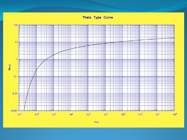
Theis’ Solution to Transient Flow Equation

Well Function W(u)

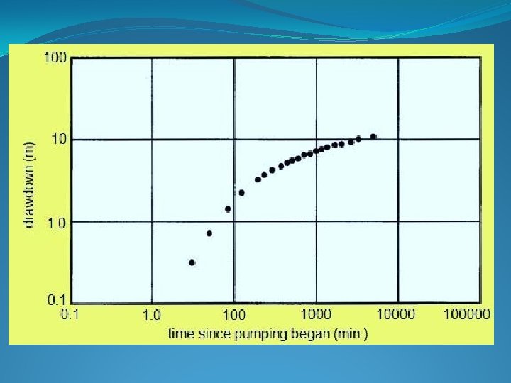
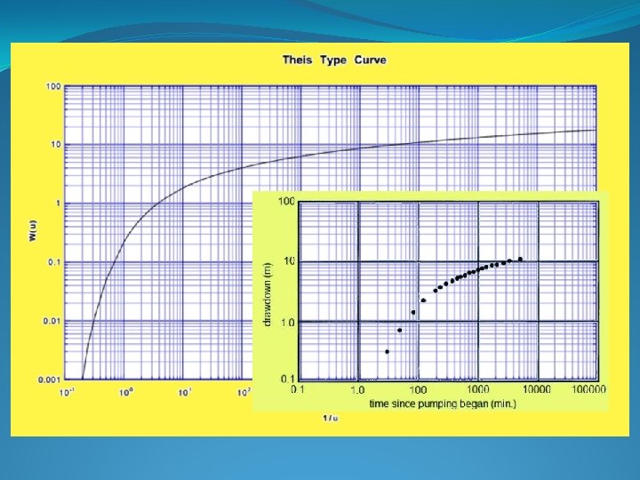
Purpose of Pumping Well Tests ØDetermine the hydraulic properties of an aquifer by performing an aquifer test in which a well is pumped at a constant rate and either the stabilized drawdown or the change in drawdown over time is measured. ØDetermine the hydraulic properties of a water well by performing variable-rate production test.

Pumping Well Terminology Q s ho h ØStatic Water Level [SWL] (ho) is the equilibrium water level before pumping commences ØPumping Water Level [PWL] (h) is the water level during pumping ØDrawdown (s = ho - h) is the difference between SWL and PWL ØWell Yield (Q) is the volume of water pumped per unit time ØSpecific Capacity (Q/s) is the yield per unit drawdown

Cone of Depression High Kh aquifer Low Kh aquifer Kh K v Ø A zone of low pressure is created centred on the pumping well Ø Drawdown is a maximum at the well and reduces radially Ø Head gradient decreases away from the well and the pattern resembles an inverted cone called the cone of depression Ø The cone expands over time until the inflows (from various boundaries) match the well extraction Ø The shape of the equilibrium cone is controlled by hydraulic conductivity

Pumping test in a completely confined aquifer

Known values: Q – pumping rate r - distance from the pumping well to the observation well (can be rw) rw – pumping well radius

Cooper-Jacob simplification

Cooper-Jacob Plot: Log(t) vs. Drawdown (s)

Cooper-Jacob Plot: Log(t) vs. Drawdown (s) to = 84 sec. Ds =0. 40 m

Cooper-Jacob Analysis 1. Fit straight-line to data (excluding early and late times if necessary): – at early times the Cooper-Jacob approximation may not be valid – at late times boundaries may significantly influence drawdown 2. Determine intercept on the time axis for s=0 3. Determine drawdown increment (Ds) for one log-cycle

Cooper-Jacob Analysis (cont. )

Recharge Effect : Recharge > Well Yield Recharge causes the slope of the log(time) vs drawdown curve to flatten as the recharge in the zone of influence of the well matches the discharge. The gradient and intercept can still be used to estimate the aquifer characteristics (T, S).

Recharge Effect : Recharge < Well Yield If the recharge is insufficient to match the discharge, the log(time) vs drawdown curve flattens but does not become horizontal and drawdown continues to increase at a reduced rate. T and S can be estimated from the first leg of the curve

Sources of Recharge ØVarious sources of recharge may cause deviation from the ideal Theis behaviour. ØSurface water: river, stream or lake boundaries may provide a source of recharge, halting the expansion of the cone of depression. ØVertical seepage from an overlying aquifer, through an intervening aquitard, as a result of vertical gradients created by pumping, can also provide a source of recharge. ØWhere the cone of depression extends over large areas, leakage from aquitards may provide sufficient recharge.

Recharge Effect: Leakage Rate High Leakage Low Leakage Recharge by vertical leakage from overlying (or underlying beds) can be quantified using analytical solutions developed by Jacob (1946). The analysis assumes a single uniform leaky bed.

Barrier Effect: No Flow Boundary Steepening of the log(time) vs. drawdown curve indicates an aquifer limited by a barrier boundary of some kind. Aquifer characteristics (T, S) can be estimated from the first leg.

Potential Flow Barriers ØVarious flow barriers may cause deviation from the ideal Theis behaviour. ØFault truncations against low permeability aquitards. ØLenticular pinchouts and lateral facies changes associated with reduced permeability. ØGroundwater divides associated with scarp slopes. ØSpring lines with discharge captured by wells. ØArtificial barriers such as grout curtains and slurry walls.

Casing Storage ØIt has been known for many decades that early time data can give erroneous results because of removal of water stored in the well casing. ØWhen pumping begins, this water is removed and the amount drawn from the aquifer is consequently reduced. ØThe true aquifer response is masked until the casing storage is exhausted. ØAnalytical solutions accounting for casing storage were developed by Papadopulos and Cooper (1967) and Ramey et al (1973) ØUnfortunately, these solutions require prior knowledge of well efficiencies and aquifer characteristics

Casing Storage Q s dp dc Schafer (1978) suggests that an estimate of the critical time to exhaust casing storage can be made more easily: tc = 3. 75 p(dc 2 – dp 2) / (Q/s) = 15 Va /Q where tc is the critical time (d); dc is the inside casing diameter (m); dp is the outside diameter of the rising main (m); Q/s is the specific capacity of the well (m 3/d/m) Va is the volume of water removed from the annulus between casing and rising main. Note: It is safest to ignore data from pumped wells earlier than time tc in wells in low-K HSU’s

Jacob-Cooper Distance-Drawdown Method ØIf more than three observation wells are used in an aquifer test, and drawdowns are measured at the same time in these wells, the Jacob distancedrawdown method can be used to determine aquifer transmissivity and storativity. ØIn this method drawdown is plotted on arithmetic scale as a function of the distance from the pumping well on the log scale. ØA straight line is then drawn through the data points and extended to the zero-drawdown axis. The intercept is the distance at which the pumping well is not affecting the water level and is designated ro

Distance-Drawdown Graph

Aquifer Characteristics

Well Efficiency Ø The efficiency of a pumped well can be evaluated using distance-drawdown graphs. Ø The distance-drawdown graph is extended to the outer radius of the pumped well (including any filter pack) to estimate theoretical drawdown for a 100% efficient well. Ø This analysis assumes the well is fully-penetrating and the entire saturated thickness is screened. Ø The theoretical drawdown (estimated) divided by the actual well drawdown (observed) is a measure of well efficiency. Ø A correction is necessary for unconfined wells to allow for the reduction in saturated thickness as a result of drawdown.

Causes of Well Inefficiency ØFactors contributing to well inefficiency (excess head loss) fall into two groups: ØDesign factors Insufficient open area of screen Poor distribution of open area Insufficient length of screen Improperly designed filter pack ØConstruction factors Inadequate development, residual drilling fluids Improper placement of screen relative to aquifer interval

Theis-Cooper-Jacob Assumptions Real aquifers rarely conform to the assumptions made for Theis-Cooper-Jacob non-equilibrium analysis Ø Isotropic, homogeneous, uniform thickness Ø Fully penetrating well Ø Laminar flow Ø Flat potentiometric surface Ø Infinite areal extent Ø No recharge The failure of some or all of these assumptions leads to “non-ideal” behavior and deviations from the Theis and Cooper-Jacob analytical solutions for radial unsteady flow

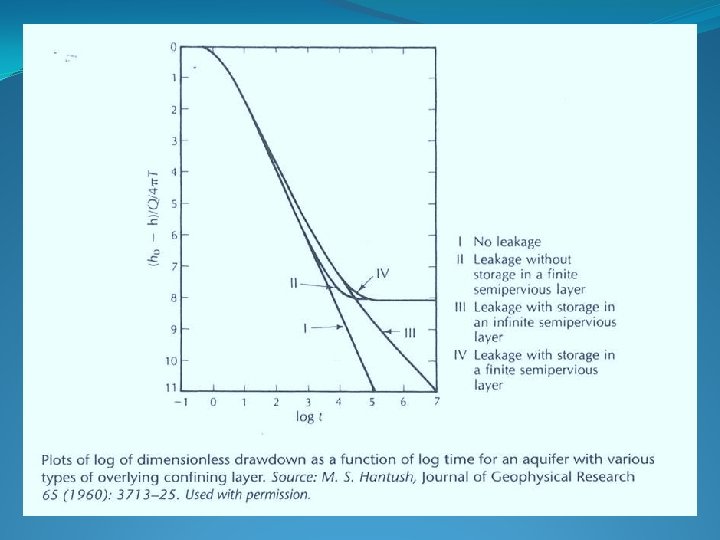
Wells in Confined Aquifers ØCompletely confined aquifer.

Wells in Confined Aquifers ØConfined, leaky with no elastic storage in the leaky layer. .

Wells in Confined Aquifers ØConfined, leaky with elastic storage in the leaky layer.

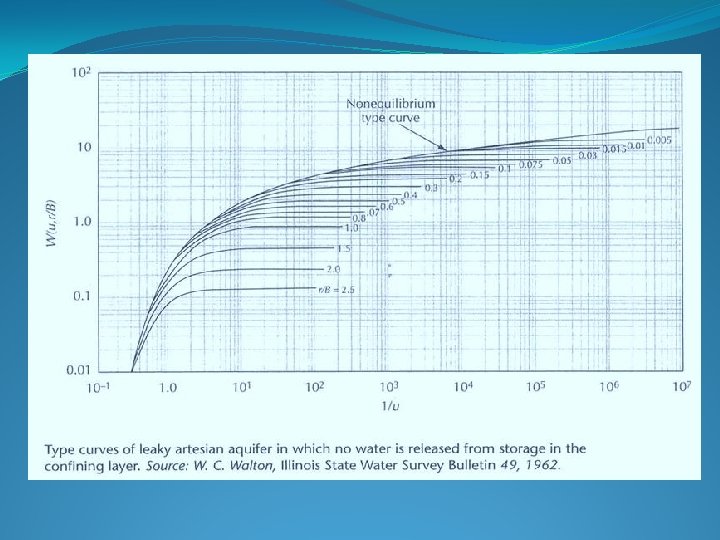
A Leaky, Confined Aquifer

A Leaky, Confined Aquifer no water drains from the confining layer (but it can drain through it) ØThe aquifer is bounded on the top by an aquitard. ØThe aquitard is overlain by an unconfined aquifer, know as the source bed. ØThe water table in the source bed is initially horizontal. ØThe water table in the source bed does not fall during pumping of the aquifer.

A Leaky, Confined Aquifer – no water drains from the confining layer ØGround water flow through the aquitard is vertical. ØThe aquifer is compressible, and water drains instantaneously with a decline in head ØThe aquitard is incompressible, so that no water is released from storage in the aquitard when the aquifer is pumped.

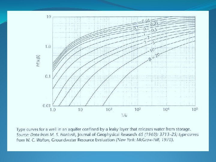
Hantush-Jacob Formula Confined with no elastic storage

Drawdown Formula Confined with elastic storage Øh 0 = initial hydraulic head (L; m or ft) Øh = hydraulic head (L; m or ft) Øh 0 – h = drawdown (L; m or ft) ØQ = constant pumping rate (L 3/T; m 3/d or ft 3/d) ØH(u, ) = a modified leaky artesian well function ØT = transmissivity (L 2/T; m 2/d or ft 2/d) Ø = r/4 B (S’/S)1/2; B = (Tb’/K’)1/2

Unconfined aquifer – 3 phases of flow to a pumping well Early stage – Øpressure drops Øspecific storage as a major contribution Øflow is horizontal Øtime-drawdown follows Theis curve

Unconfined aquifer – 3 phases of flow to a pumping well Second stage – Øwater table declines Øspecific yield as a major contribution Øflow is both horizontal and vertical Øtime-drawdown is a function of Kv/Kh r, b

Unconfined aquifer – 3 phases of flow to a pumping well Later stage – Ørate of drawdown decreases Øflow is again horizontal Øtime-drawdown again follows Theis curve ØS - the specific yield.

Neuman’s assumptions ØAquifer is unconfined. ØVadose zone has no influence on the drawdown. ØWater initially pumped comes from the instantaneous release of water from elastic storage. ØEventually water comes from storage due to gravity drainage of interconnected pores.

Neuman’s assumptions (cont. ) ØThe drawdown is negligible compared to the saturated thickness. ØThe specific yield is at least 10 times the elastic storativity. ØThe aquifer may be – but does not have to be – anisotropic with the radial hydraulic conductivity different than the vertical hydraulic conductivity.

Drawdown Formula unconfined with elastic storage

Neuman’s type curves

Aquifer Test Software http: //trials. swstechnology. com/demos/Aquifer. Test_Pro/Aquifer. Test_ Pro-Trial. msi

Partial Penetration ØPartial penetration effects occur when the intake of the well is less than the full thickness of the aquifer

Effects of Partial Penetration Ø The flow is not strictly horizontal and radial. Ø Flow-lines curve upwards and downwards as they approach the intake and flow-paths are consequently longer. Ø The convergence of flow-lines and the longer flow-paths result in greater head-loss than predicted by the analytical equations. Ø For a given yield (Q), the drawdown of a partially penetrating well is more than that for a fully penetrating well. Ø The analysis of the partially penetrating case is difficult but Kozeny (1933) provides a practical method to estimate the change in specific capacity (Q/s).

Q/s Reduction Factors

Q/s Reduction Factors Example

Partial Penetration Alternative ØMultiple screened sections distributed over the entire saturated thickness functions more efficiently for the same open area.

Screen Design 300 mm diameter well with single screened interval of 15 m in aquifer of 30 m thickness; L/b = 0. 5 and 2 L/r = 200 F = 0. 5 × {1 + 7 x cos(0. 5 p/2) (1/200)} = 0. 67 300 mm diameter well with 5 x 3 m solid sections alternating with 5 x 3 m screened sections, in an aquifer of 30 m thickness; there effectively are five aquifers. L/b = 0. 5 and 2 L/r = 40 F = 0. 5 × {1 + 7 × cos(0. 5 p/2) (1/40)} = 0. 89 This is clearly a much more efficient well completion.

Recovery Data Ø When pumping is halted, water levels rise towards their pre-pumping levels. Ø The rate of recovery provides a second method for calculating aquifer characteristics. Ø Monitoring recovery heads is an important part of the well-testing process. Ø Observation well data (from multiple wells) is preferable to that gathered from pumped wells. Ø Pumped well recovery records are less useful but can be used in a more limited way to provide information on aquifer properties.

Recovery Curve Drawdown 10 m Recovery 10 m Pumping Stopped The recovery curve on a linear scale appears as an inverted image of the drawdown curve. The dotted line represent the continuation of the drawdown curve.

Superposition Ø The drawdown (s) for a well pumping at a constant rate (Q) for a period (t) is given by:

Superposition Drawdown 10 m Recovery 10 m Pumping Stopped

Residual Drawdown and Recovery

Time-Recovery Graph to’ = 0. 12 hrs Dsr = 4. 6 m Aquifer characteristics can be calculated from a log(time)recovery plot but the drawdown (s) curve for the pumping phase must be extrapolated to estimate recovery (s - s’)

Time-Recovery Analysis

Time-Residual Drawdown Graph Ds’ = 5. 2 m Transmissivity can be calculated from a log(time ratio)residual drawdown (s’) graph by determining the gradient. For such cases, the x-axis is log(t/t’) and thus is a ratio.

Time-Residual Drawdown Analysis

Residual Drawdown for Real Aquifers Ø Theoretical intercept is 1 Ø >> 1 indicates a recharge effect Ø >1 may indicate greater S for pumping than recovery ? consolidation Ø < 1 indicates incomplete recovery of initial head - finite aquifer volume Ø << 1 indicates incomplete recovery of initial head - small aquifer volume

DST Drill Stem Valve Packer Perforated Section Packer Gauge Ø The drill stem test, used widely in petroleum engineering, is a recovery test. Ø Packers are used to isolate the HSU of interest which has been flowing for some time. Ø Initially the bypass valve is open allowing free circulation. Ø When the bypass valve is closed, the formation pressure is “shut-in” and begins to recover towards the static value. Ø The Horner plot is a direct analogue of the residual drawdown plot.

DST Analysis p (k. Pa) po Dp 100 10 t / t’ 1

Slug Test Displaced Head Displacer Ø The recovery test in a borehole after withdrawal or injection (or displacement) of a known volume of water is called a slug test. Ø The slug test is a rapid field method for estimation of moderate to low K-values in a single well. Ø The procedure is: Ø initial head is noted Ø the slug is removed, added or displaced Initial Head instantaneously (displacement is best in this respect) Ø head recovery is monitored (usually with a submerged pressure logging device) Ø typical head changes are 2 -3 m in 25 -50 mm diameter piezometers so the volume of the slug is typically only 1 -10 liters

Slug Analysis Tube or Casing 2 ra L 2 rw Ø ra is access tube internal radius Ø rw is perforated section external radius Ø L is length of perforated section Ø ho is initial head, t = to Ø h(t) is head after recovery time t Ø A is the tube or casing open area = pra 2 ØF is a shape factor = 2 p. L/ln(L/rw) Ø Analysis methods include: Ø Hvorslev (1951) Ø Cooper et al (1967) Ø The Cooper analysis considers storage but the Hvorslev analysis is more widely used.

Hvorslev Analysis Tube or Casing 2 ra 1. 0 0. 9 0. 8 0. 7 0. 6 0. 5 h 0. 4 ho To 0. 3 0. 2 L 0. 1 2 rw Time, t - to

Bounded Aquifers ØSuperposition was used to calculate well recovery by adding the effects of a pumping and recharge well starting at different times. ØSuperposition can also be used to simulate the effects of aquifer boundaries by adding wells at different positions. ØFor boundaries, the wells that create the same effect as a boundary are called image wells. ØThis relatively simple application of superposition for analysis of aquifer boundaries was for described by Ferris (1959)

Image Wells Ø Recharge boundaries at Ø Barrier boundaries at distance (r) are simulated by by a recharge image well at a pumping image well at an an equal distance (r) across the boundary. r r

General Solution ri r rp r Ø For a barrier boundary, for all points on the boundary rp = ri and the drawdown is doubled. Ø For a recharge boundary, for all points on the boundary rp = ri and the drawdown is zero.

Specific Solutions For the barrier boundary case: a = (ri/rp)2 and 0<a<1 For the recharge boundary case: a = (ri/rp)2 and 0<a<1

Multiple Boundaries A recharge boundary and a barrier boundary at right angles can be generated by two pairs of pumping and recharge wells. Two barrier boundaries at right angles can be generated by superposition of an array of four pumping wells. r 2 r 1

Parallel Boundaries A parallel recharge boundary and a barrier boundary (or any pattern with parallel boundaries) requires an infinite array of image wells. r 1 r 2

Boundary Location Ø For an observation well at distance r 1, measure off the same drawdown (s), before and after the “dog leg” on a log(time) vs. drawdown plot. Ø Find the times t 1 and t 2. s t 1 s t 2 Ø Assuming that the “dog leg” is created by an image well at distance r 2 , if the drawdowns are identical then W(u 1) = W(u 2) so u 1 = u 2. Thus: r 12 S/4 Tt 1 = r 22 S/4 Tt 2 r 12 t 2 = r 22 t 1 and r 2 = r 1(t 2 / t 1)½ Ø The distance r 2=the radial distance from the observation point to the boundary. Ø Repeating for additional observation wells may help locate the boundary.