Applied Fluvial Geomorphology Week 2 With thanks to

Applied Fluvial Geomorphology Week 2 With thanks to David Montgomery (UW Seattle) Peter Wilcock (JHU) Matt Kondolf (UCB) Karen Gran (UMD)

Eight themes 1. 2. 3. 4. 5. 6. 7. 8. Drainage basin & hydrology (discharge) Channel pattern Channel x-sectional geometry & slope Grain size & sediment transport regime Flood plain & relation to channel Biota: in channel & flood plain Engineered structures History and context

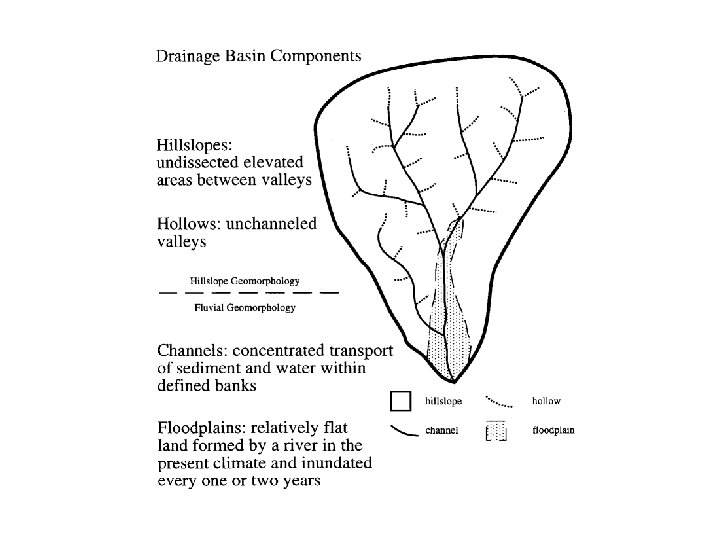
Definitions Drainage Basin: The drainage area which contributes water to a particular channel or set of channels. Synonymous with watershed (America) and catchment (everywhere else). NB: there are many ‘sheds’, and generally they may not coincide with the watershed: groundwater-shed nutrient-shed propagule-shed

Structure of drainage basins Strahler stream ordering Stream order Number of segments 1 9 2 3 3 1

Drainage basins Lmax ~ A 0. 6 Hack’s Law Lmax : length of longest stream Horton’s Laws Order, w Number Average of Length Area Streams (km) (km 2) 1 60 2 5 2 13 5 12 3 9 13 40 4 4 20 110 5 1 55 330 Ni: number of stream segments of order i Li: mean length of stream segments of order i

Drainage basins are the “type fractal” – strong selfsimilarity provides a basis for prediction (we hope!) log P( A > a ) Brushy River Basin (ALABAMA) Upper Rio Salado basin, NM courtesy Kelly Caylor & Ignacio Rodriguez-Iturbe log a [km 2]

Key watershed points • Land use: agriculture, grassland, forest… • Urbanization • Water pathways to stream: drain tiles, parking lots, ditches & culverts • Nutrient sources: mainly N, P • Gradient & physiography • Lithology • AND DON’T LOOK ONLY UPSTREAM! Class discussion points: sources of watershed information; intro to USGS gage information http: //water. usgs. gov/

River Channels A channel has two basic functions within a drainage basin. It must convey : 1. all of the WATER, and 2. some or all of the SEDIMENT 1 --that the drainage basin delivers by the various runoff and hillslope processes. To do this, the channel adjusts itself to a particular slope and geometry ( width, depth, sinuosity, and distribution of small-scale features like pools and bars) Major point 1: it’s a river of water and a river of sediment! Major point 2: in general it’s much harder to move sediment than water. Beyond the fundamental "tasks" of moving water and sediment, the form of the channel will also be affected . locally, by bank vegetation, fallen trees, bank sediments, tributary inputs, and bank modifications; . systemically, by the progressive inclusion of increasing tributary areas with their own particular influxes of water and sediment; and . temporally, by the sporadic disturbances to a watershed occasioned by large storms, fires, or human activity. Our study of channel geomorphology is the understanding of how these factors affect channel form, and how to interpret or to predict that form even with less-than-perfect information. 1 depending on whether the river is net depositional (e. g. lowlands/deltaic river channels)

Two main types of channels Alluvial channels Channels formed in and by sediment transported by the river (= "alluvium") under its current hydrologic and climatologic regime (and so could be transported again). These “self-formed channels” are free to adjust their shape in response to changes in flow. Non-alluvial channels Channels not formed in alluvium, such as- • bounded by bedrock or concrete; • deeply incised into bedrock; • choked by relatively immovably objects such as logs or boulders or landslide sediment; • rimmed with thick and deeply rooted bank vegetation; • channels that have "inherited" a valley geometry from some other geologic process (such as glaciation) in the recent past; or • channels that have undergone a significant change in hydrologic regime (as a result of diversion or watershed disturbance) Copyright © J. Michael Daniels 2002 self adjusting container USFWS imposed container

Steep channel morphologies Step-pool

Steep channel morphologies Step-pool

Steep channel morphologies Pool-riffle

Lower-gradient channels STRAIGHT CHANNELS are naturally uncommon in alluvial channels because unless they are narrow relative to their depth (b/h <~ 20) they are inherently unstable: any minor perturbation of the flow, such as caused by a hard projection or a bump in the bank, will tend to establish the oscillation of the thalweg that leads to concentrated scour of pools, point-bar formation, and a meandering pattern. Delta distributary channels are often straight, however. BRAIDED CHANNELS have flow divided into more than one thread. Island width is comparable to channel width. Rates of local lateral shifting and local bank erosion are generally greater than meandering channels.

Lower-gradient channels BRAIDED CHANNELS Sunwapta, Alberta Rakaia, NZ Aichilik, AK

Lower-gradient channels MEANDERING: The most common type of channel, where the main thread of the flow (the thalweg) oscillates from one side of the channel to the other. Pools and riffles form in predictable locations along meandering rivers, which become more precisely fixed in place as the magnitude of the meanders increases. In most natural meandering channels the ratio of channel length to straight-line downvalley distance lies between 1. 5 and 2. Where this ratio, called the sinuosity, is less than 1. 3 the channel is not termed "meandering" but instead is "sinuous" or "straight. "

Lower-gradient channels MEANDERING: The most common type of channel, where the main thread of the flow (the thalweg) oscillates from one side of the channel to the other. Mississippi (Fisk) Pembina, Alberta

Lower-gradient channels Strickland (Wes Lauer)

Lower-gradient channels ANASTOMOSED OR ANABRANCHING CHANNELS Saskatchewan River

Stream type (Schumm)

Montgomery & Buffington (1993)

Rosgen classification

Kuroki-Kishi: braiding vs meandering

Stream plan pattern summary • You can’t use a purely mechanistic approach because we still don’t fully understand what controls stream width and plan pattern BUT • You can’t just use descriptive classifications either because channel geometry and plan pattern can change, and do respond to changes in partly predictable ways • Message: use both approaches, and know their limits!

Stability vs dynamism The default behavior of natural river channels is migration and change. In general stability is not natural Unless the channel is incised, bank erosion is more-or-less balanced by accretion or deposition on the floodplain. Bank stabilization is one of the primary reasons people do stream restoration work, but bank stabilization alone does not make sense. There needs to be another reason (i. e. protect property).

Rivers record evidence of change Pembina Fisk, Mississippi River

Rivers record evidence of change Red River of the North, MN Watownwan River

Rivers record evidence of change Riviere des Ha!Ha!, QU Niobrara River, NE (D. Jerolmack)

Some general trends • In general, incision narrowing, deposition widening • Bedrock rivers: high rates of incision and/or stronger lithologies steeper, narrower channels [step-pool, cascade] • Alluvial rivers: width ~ bed-material transport rate; vegetation and/or strong banks act to reduce width • Meandering vs braiding mainly controlled by b/h (threshold ~50 -100)

Floodplains and Terraces A floodplain is the surface that has been built up next to a river channel under the current hydrologic and sedimentological regime. It is composed of alluvium, the sediment carried by the river. In contrast, a terrace is also a constructed surface and also underlain by alluvium, but it has not formed under the current regime of the river. Instead it represents floodplain formation at an earlier time when, for whatever reasons, deposition was occurring at a higher elevation. Copyright © Keith Richards 2002

Floodplain formation 3 Basic processes for floodplain formation 1. Lateral accretion 2. Overbank deposition 3. Patchwork mosaic driven by LWD

Features associated with floodplain construction: From lateral migration: Oxbow lakes Scroll bars Wetlands Side channels Point bars Cutbanks Ridge-swale topography Vegetation age gradients From overbank deposition: Natural levees Backwater swamps Splay deposits From LWD patchwork: Side channels Patchy vegetation ages Complex topography Copyright © Richard Kesel 2002

Floodplain detachment Erosion control levee has broken connection between channel & floodplain

Erosion & floodplain detachment Artificial drainage & straightening leading to incision and loss of floodplain connection, Clay Co. Minnesota

Intro to quantitative methods to the blackboard!

The basic equations

The basic equations

Alternative drag estimation

References: Manning’s n • • • Copeland, Ronald R. , 2000. Determination of flow resistance coefficients due to shrubs and woody vegetation. US Army Corps of Engineers Dudley, Syndi J. ; Fischenich, J. Craig; and Abt, Steven R. , 1998. Effect of woody debris entrapment on flow resistance. Journal of the American Water Resources Association, pp. 1189 -1197. Fischenich, Dr. Craig; 2000. Robert Manning (A Historical Perspective) http: //el. erdc. usace. army. mil/elpubs/pdf/sr 10. pdf Freeman, Gary E. ; Copeland, Ronald R. ; Rahmeye, William; and Derrick, David L. , Field determination of Manning’s n value for shrubs and woody vegetation. Hessel, Rudi, Jetten, Victor, Guanghui, Zhang. 2003. Estimating Manning’s n for steep slopes. Elsevier Science B. V. Jarvela, Juha. 2004. Determination of flow resistance caused by non-submerged woody vegetation. Laboratory of Water Resources, Helsinki University of Technology. Jarvela, J. . 2002. Determination of flow resistance of vegetated channel banks and floodplains. Laboratory of Water Resources, Helsinki University of Technology. Khoury, Fadi; 2005. History of the Manning Formula. http: //manning. sdsu. edu Marcus, W. Andrew; Roberts, Keith; Harvey, Leslie; and Tackman, Gary. 1992. An evaluation of methods for estimating Manning’s n in small mountain streams. Department of Earth Sciences, Montana State University. Tinkler, K. J. . 1996. Critical flow in rockbed streams with estimated values for Manning’s n. Department of Geography, Brock University, St. Catherines, On.

Example calculated rating data Darcy-Weisbach Manning

Hydraulic geometry: downstream Note apparent powerlaw behavior, suggesting: B = a. Qb h = c. Qf U = k. Qm [what must be true of b, f, m? ]

Hydraulic geometry: downstream Note apparent powerlaw behavior, suggesting: B = a. Qb h = c. Qf U = k. Qm [what must be true of b, f, m? ] Dodov & Foufoula-Georgiou, 2004

Hydraulic geometry B = a. Qb h = c. Qf U = k. Qm Plots like this in which the variable is time at a fixed location are called “at a station” HG What controls this?

Hydraulic geometry: at a station Note apparent powerlaw behavior, suggesting: B = a. Qb h = c. Qf U = k. Qm [what must be true of b, f, m? ]

Hydraulic geometry B = a. Qb h = c. Qf U = k. Qm Here we compare at a station with downstream HG What is going on here?

Hydraulic geometry Typical at a station values (midwestern streams) b = 0. 25 B = a. Qb f h = c. Qf = 0. 4 m = 0. 35 Typical downstream values b = 0. 5 f = 0. 4 m = 0. 1 U = k. Qm

Homework: Make a spreadsheet that calculates discharge through a single topographic cross section for a given value of cf or Manning’s n and a channel slope S, as a function of water-surface elevation (“stage”). Use it to investigate how stage-discharge curves depend on S and n (or cf ). Beginner level: assume a rectangular cross section in which b>>h Advanced level: let the user enter arbitrary cross-sectional topography Extra-galactic level: let the roughness also vary over the section

General controls on slope • Flow depth and shear stress: given = gh. S, small h (small Qw) higher S to move bed sediment • In alluvial rivers, S ~ Qs/Qw

Longitudinal profile Most rivers are concave in long profile, i. e. the slope decreases downstream Contributing factors? How do you expect the dependent variables in the basic equations to change downstream? Why?

Longitudinal profile Chin (1999) S. Monica Mtns Hack (1957) Virginia Contributing factors? How do you expect the dependent variables in the basic equations to change downstream? Why? Wegmann & Pazzaglia (2002) Washington

Long profile Minnesota River, from mrbdc. mnsu. edu

Natural, mostly stochastic variability

Variability in morphology Compare these: what is the difference between the natural and artificial meanders?

Distribution of step pool spacing Chin (2002)

Distribution of step pool spacing Chin (2002)

Distribution of step-pool geometry Zimmerman & Church (2001)

Distribution of step-pool geometry Zimmerman & Church (2001)

Moody & Troutman 2002 Local avg depth/reach avg depth Surface width/mean surface width Natural variability of width & depth

Moody & Troutman 2002 Local avg depth/reach avg depth Surface width/mean surface width Natural variability of width & depth

Distribution of curvature Williams (1986)

References Chin, A. (2002), The periodic nature of step-pool mountain streams, Am J Sci, 302, 144 -167. Moody, J. A. , and B. M. Troutman (2002), Characterization of the spatial variability of channel morphology, Earth Surface Processes and Landforms, 27, 1251 -1266. Williams, G. P. (1986), River meanders and channel size, Journal of Hydrology, 88, 147 -164. Zimmermann, A. , and M. Church (2001), Channel morphology, gradient profiles and bed stresses during flood in a step-pool channel, Geomorphology, 40, 311 -327.

Variable discharge: which one to use? Partial record, USGS Anoka Gage

Variable discharge: which one to use? Bankfull refers to the elevation at which the water in the channel spills out of its banks and enters the floodplain. The bankfull discharge refers to the discharge at which this happens. How do you determine bankfull? 1) Height of “valley flat”. 2) Location of cross-sectional slope break. 3) Region inundated in 1 -2 year flood. 4) Location that provides minimum width: depth ratio (Williams, 1978). Karen Gran, UMD

Bankfull also can be determined from hydrologic data. As the stage (depth) rises, the relationship between stage and discharge changes at the point where water spills out of its banks. Thus the slope break on a stage-discharge curve represents bankfull stage. Karen Gran, UMD Bankfull Stage at Break in Slope From W. Lauer

There is a lot of talk about bankfull discharge, especially in the stream restoration community. Why is bankfull so important? Should so much weight be placed on bankfull flow? Let’s step back and ask the question: What discharge forms channels? This is known as the effective discharge. Maximum sediment transport occurs at relatively high-frequency, low-magnitude events. Karen Gran, UMD From Wolman and Miller, 1960

Likewise, bankfull flows seem to occur relatively frequently – Q 1. 5 - Q 2 (1. 5 -year to 2 year flood events, for temperate, perennial rivers only). These are high-frequency, low-magnitude events. Karen Gran, UMD

Can we link the max sediment discharge to the effective discharge or to the bankfull discharge? Andrews (1980) measured effective discharge and found a tight correlation between effective discharge and bankfull discharge.

So now we have a field case showing bankfull occurs ~ Q 1. 5 to Q 2, and another field case showing a link between bankfull discharge and maximum sediment transport/effective discharge. This is great, because now there is a feature you can measure in the field (bankfull depth), and it relates to the discharge with maximum sediment transport. You can thus design a channel for bankfull flow, and know you are hitting the channel-forming discharge… BUT WAIT There a number of cases where, even in an alluvial river, the bankfull discharge does not correspond to anything close to Q 1. 5 – Q 2, and this is important to know in stream restoration! Karen Gran, UMD

Remember the study by Williams (1978): Although the peak in frequency distribution corresponds to Qbf of ~1. 25 – 2, many bankfull flows were outside of this range Nash (1994) found that “the observed recurrence interval of the effective discharge… is highly variable, ranging from a week to several decades, calling into question the widely held notion that effective discharge occurs about once a year. ”

So although we generally assume as an average that Bankfull Discharge = Effective channel-forming Discharge = 1. 5 -2 -year flood event There are many exceptions, especially streams where… 1) Land use has altered hydrologic regime, changing flood peak timing and magnitude 2) Streams occupy valleys formed in a different hydrologic regime (e. g. streams occupying glacially-derived valleys…) 3) Flows are strongly influenced by features unrelated to simple flow and sediment transport (such as large woody debris, structures, concrete, etc. ) You really need to assess the history of a channel. It is not smart to simply take a bankfull measurement and assume that corresponds to a 1. 5 – 2 year flood event. We’ll talk more about discharge statistics and bankfull flows when we look into stream hydrology Karen Gran, UMD