Applied Bayesian Methods Phil Woodward 2014 1 Introduction

Applied Bayesian Methods Phil Woodward 2014 1

Introduction to Bayesian Statistics Phil Woodward 2014 2

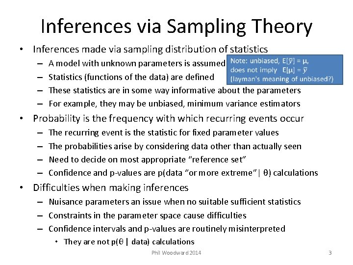
Inferences via Sampling Theory • Inferences made via sampling distribution of statistics – – A model with unknown parameters is assumed Statistics (functions of the data) are defined These statistics are in some way informative about the parameters For example, they may be unbiased, minimum variance estimators • Probability is the frequency with which recurring events occur – – The recurring event is the statistic for fixed parameter values The probabilities arise by considering data other than actually seen Need to decide on most appropriate “reference set” Confidence and p-values are p(data “or more extreme”| θ) calculations • Difficulties when making inferences – Nuisance parameters an issue when no suitable sufficient statistics – Constraints in the parameter space cause difficulties – Confidence intervals and p-values are routinely misinterpreted • They are not p(θ | data) calculations Phil Woodward 2014 3

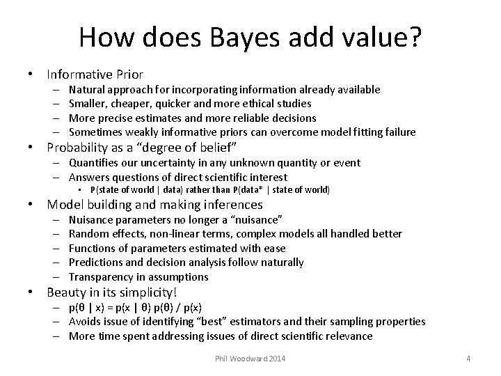
How does Bayes add value? • Informative Prior – – Natural approach for incorporating information already available Smaller, cheaper, quicker and more ethical studies More precise estimates and more reliable decisions Sometimes weakly informative priors can overcome model fitting failure • Probability as a “degree of belief” – Quantifies our uncertainty in any unknown quantity or event – Answers questions of direct scientific interest • P(state of world | data) rather than P(data* | state of world) • Model building and making inferences – – – Nuisance parameters no longer a “nuisance” Random effects, non-linear terms, complex models all handled better Functions of parameters estimated with ease Predictions and decision analysis follow naturally Transparency in assumptions • Beauty in its simplicity! – p(θ | x) = p(x | θ) p(θ) / p(x) – Avoids issue of identifying “best” estimators and their sampling properties – More time spent addressing issues of direct scientific relevance Phil Woodward 2014 4

Probability • Most Bayesians treat probability as a measure of belief – Some believe probabilities can be objective (not discussed here) – Probability not restricted to recurring events • E. g. probability it will rain tomorrow is a Bayesian probability – Probabilities lie between 0 (impossible event) and 1 (certain event) – Probabilities between 0 and 1 can be calibrated via the “fair bet” • What is a “fair bet”? – Bookmaker sells a bet by stating the odds for or against an event – Odds are set to encourage a punter to buy the bet • E. g. odds of 2 -to-1 against means that for each unit staked two are won, plus the stake – A fair bet is when one is indifferent to being bookmaker or punter • i. e. one doesn’t believe either side has an unfair advantage in the gamble Phil Woodward 2014 5

Probability • Relationship between odds and probability – One-to-one mapping between odds (O) and probability (P) Where O equals the ratio X/Y for odds of X-to-Y in favour and the ratio Y/X for odds of X-to-Y against an event e. g. odds of 2 -to-1 against, if fair, imply probability equals ⅓ • Probabilities defined this way are inevitably subjective – – – People with different knowledge may have different probabilities Controversy occurs when using this definition to interpret data Science should be “objective”, so “subjectivity” to some is heresy But where do the models that Frequentists use come from? Are the decisions made when designing studies purely objective? Is judgment needed when generalising from a sample to a population? Phil Woodward 2014 6

Probability • Subjectivity does not mean biased, prejudiced or unscientific – Large body of research into elicitation of personal probabilities – Where frequency interpretation applies, these should support beliefs • E. g. the probability of the next roll of a die coming up a six should be ⅙ for everyone unless you have good reason to doubt the die is fair – An advantage of the Bayesian definition is that it allows all other information to be taken into account • E. g. you may suspect the person offering a bet on the die roll is of dubious character • Bayesians are better equipped to win at poker than Frequentists! • All unknown quantities, including parameters, are considered random variables Epistemic uncertainty – each parameter still has only one true value – our uncertainty in this value is represented by a probability distribution Phil Woodward 2014 7

Exchangeability • Exchangeability is an important Bayesian concept – exchangeable quantities cannot be partitioned into more similar sub-groups – nor can they be ordered in a way that infers we can distinguish between them – exchangeability often used to justify prior distribution for parameters analogous to classical random effects Phil Woodward 2014 8

The Bayesian Paradigm From A and B comes Bayes Theorem Nothing controversial yet. Phil Woodward 2014 9

The Bayesian Paradigm How is Bayes Theorem (mis)used? Coin tossing study: Is the coin fair? Model ri ~ bern(π) i = 1, 2, . . . , n ri = 1 if ith toss a head, = 0 if a tail Let terms in Bayes Theorem be A = π (controversial) B = r then Phil Woodward 2014 Why? 10

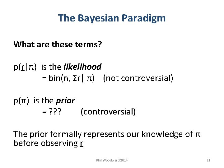
The Bayesian Paradigm What are these terms? p(r|π) is the likelihood = bin(n, Σr| π) (not controversial) p(π) is the prior = ? ? ? (controversial) The prior formally represents our knowledge of π before observing r Phil Woodward 2014 11

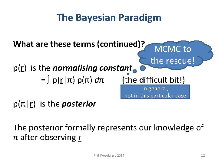
The Bayesian Paradigm What are these terms (continued)? MCMC to the rescue! p(r) is the normalising constant = ∫ p(r|π) p(π) dπ (the difficult bit!) p(π|r) is the posterior In general, not in this particular case The posterior formally represents our knowledge of π after observing r Phil Woodward 2014 12

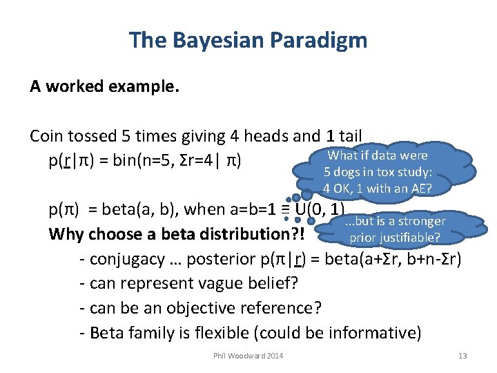
The Bayesian Paradigm A worked example. Coin tossed 5 times giving 4 heads and 1 tail What if data were p(r|π) = bin(n=5, Σr=4| π) 5 dogs in tox study: 4 OK, 1 with an AE? p(π) = beta(a, b), when a=b=1 ≡ U(0, 1). . . but is a stronger Why choose a beta distribution? ! prior justifiable? - conjugacy … posterior p(π|r) = beta(a+Σr, b+n-Σr) - can represent vague belief? - can be an objective reference? - Beta family is flexible (could be informative) Phil Woodward 2014 13

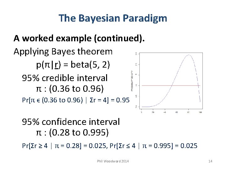
The Bayesian Paradigm A worked example (continued). Applying Bayes theorem p(π|r) = beta(5, 2) 95% credible interval π : (0. 36 to 0. 96) Pr[π ϵ (0. 36 to 0. 96) | Σr = 4] = 0. 95 95% confidence interval π : (0. 28 to 0. 995) Pr[Σr ≥ 4 | π = 0. 28] = 0. 025, Pr[Σr ≤ 4 | π = 0. 995] = 0. 025 Phil Woodward 2014 14

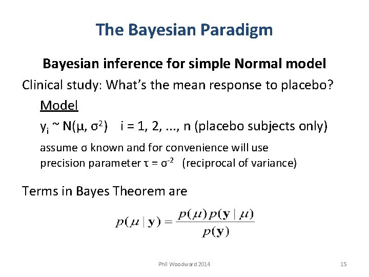
The Bayesian Paradigm Bayesian inference for simple Normal model Clinical study: What’s the mean response to placebo? Model yi ~ N(µ, σ2) i = 1, 2, . . . , n (placebo subjects only) assume σ known and for convenience will use precision parameter τ = σ-2 (reciprocal of variance) Terms in Bayes Theorem are Phil Woodward 2014 15

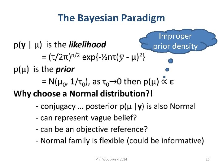
The Bayesian Paradigm Improper prior density Phil Woodward 2014 16

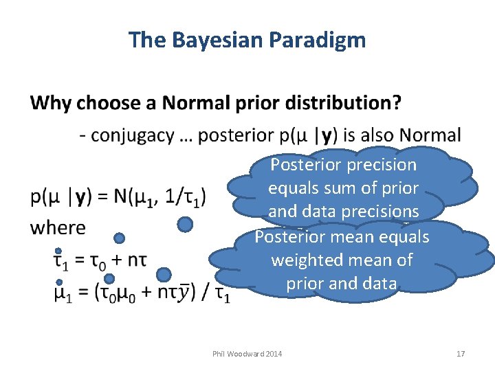
The Bayesian Paradigm Posterior precision equals sum of prior and data precisions Posterior mean equals weighted mean of prior and data Phil Woodward 2014 17

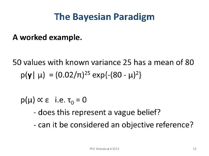
The Bayesian Paradigm Phil Woodward 2014 18

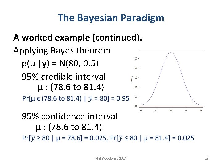
The Bayesian Paradigm A worked example (continued). Applying Bayes theorem p(µ |y) = N(80, 0. 5) 95% credible interval µ : (78. 6 to 81. 4) 95% confidence interval µ : (78. 6 to 81. 4) Phil Woodward 2014 19

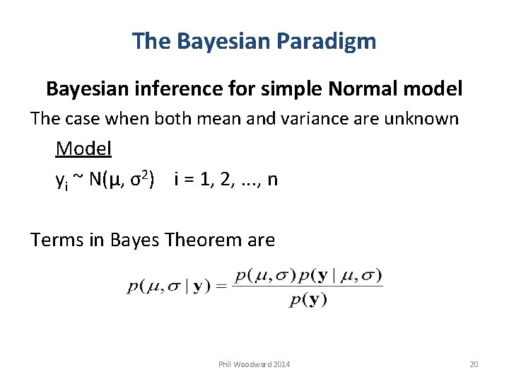
The Bayesian Paradigm Bayesian inference for simple Normal model The case when both mean and variance are unknown Model yi ~ N(µ, σ2) i = 1, 2, . . . , n Terms in Bayes Theorem are Phil Woodward 2014 20

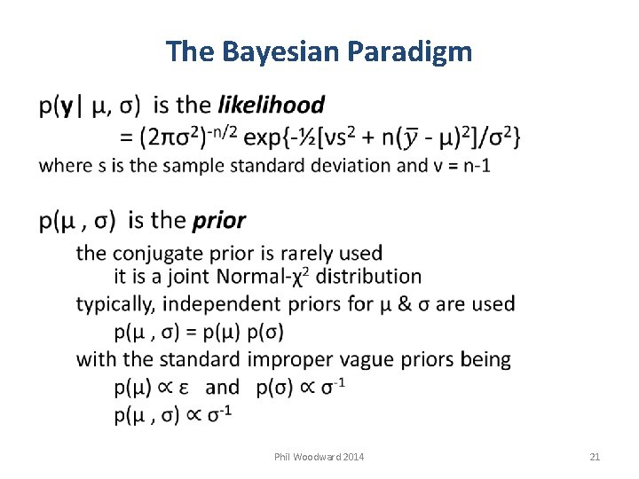
The Bayesian Paradigm Phil Woodward 2014 21

The Bayesian Paradigm Phil Woodward 2014 22

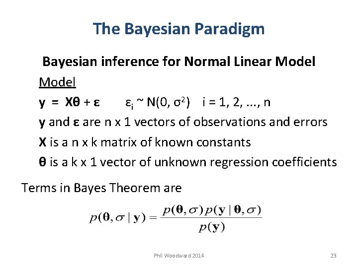
The Bayesian Paradigm Bayesian inference for Normal Linear Model y = Xθ + ε εi ~ N(0, σ2) i = 1, 2, . . . , n y and ε are n x 1 vectors of observations and errors X is a n x k matrix of known constants θ is a k x 1 vector of unknown regression coefficients Terms in Bayes Theorem are Phil Woodward 2014 23

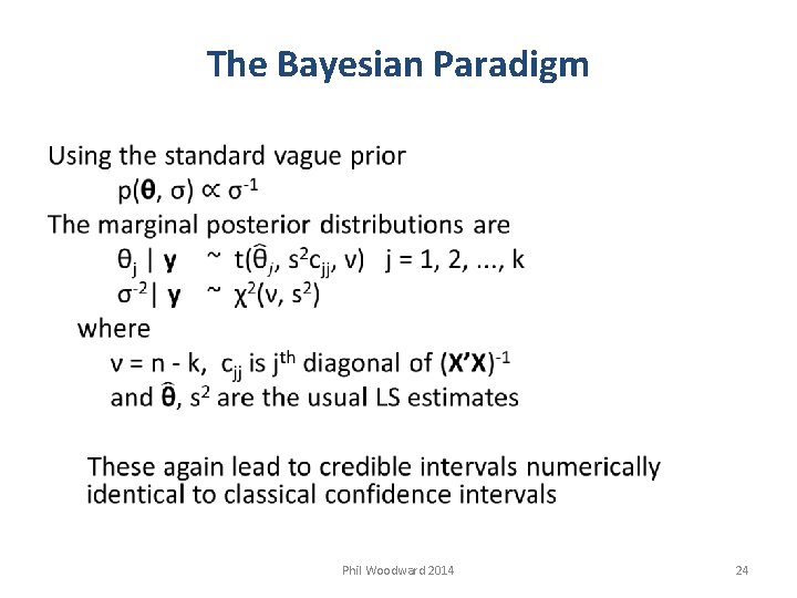
The Bayesian Paradigm Phil Woodward 2014 24

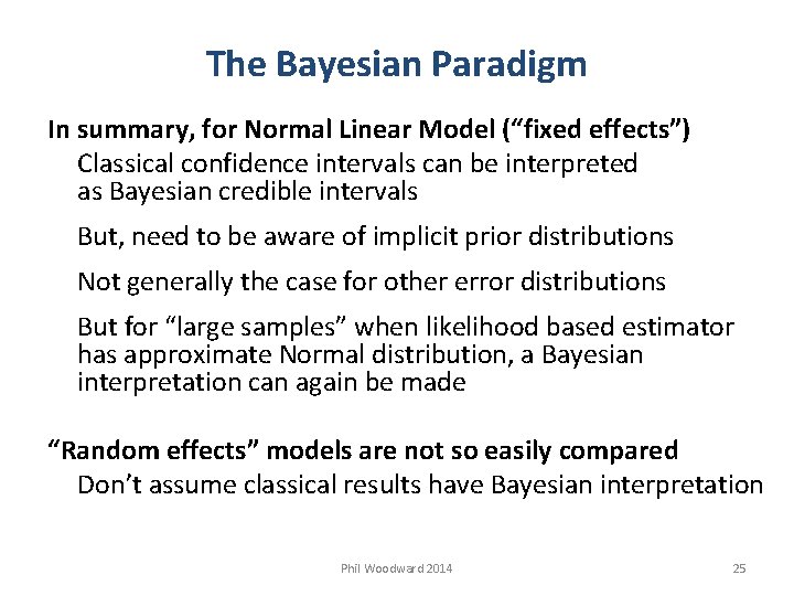
The Bayesian Paradigm In summary, for Normal Linear Model (“fixed effects”) Classical confidence intervals can be interpreted as Bayesian credible intervals But, need to be aware of implicit prior distributions Not generally the case for other error distributions But for “large samples” when likelihood based estimator has approximate Normal distribution, a Bayesian interpretation can again be made “Random effects” models are not so easily compared Don’t assume classical results have Bayesian interpretation Phil Woodward 2014 25

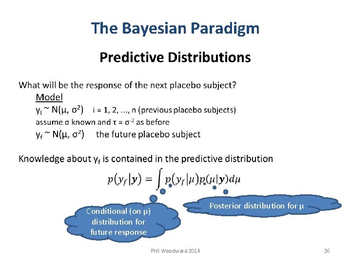
The Bayesian Paradigm Conditional (on µ) distribution for future response Phil Woodward 2014 Posterior distribution for µ 26

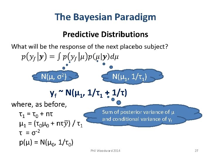
The Bayesian Paradigm N(µ, σ2) N(µ 1, 1/τ1) yf ~ N(µ 1, 1/τ1 + 1/τ) Sum of posterior variance of µ and conditional variance of yf Phil Woodward 2014 27

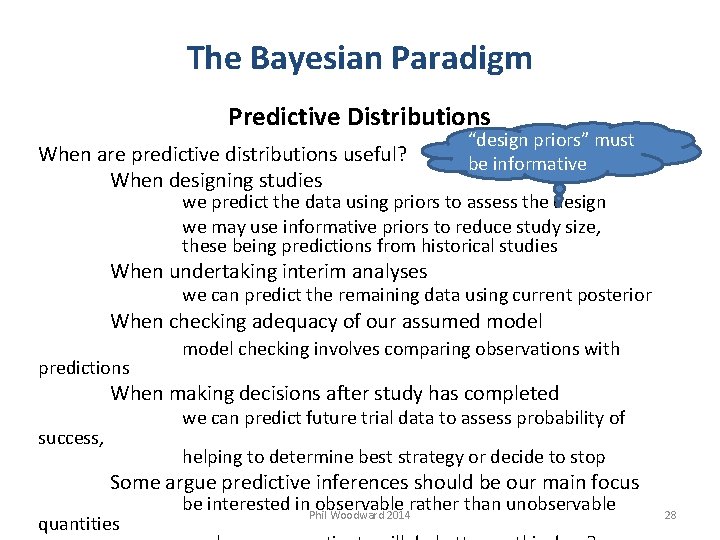
The Bayesian Paradigm Predictive Distributions When are predictive distributions useful? When designing studies “design priors” must be informative we predict the data using priors to assess the design we may use informative priors to reduce study size, these being predictions from historical studies When undertaking interim analyses we can predict the remaining data using current posterior When checking adequacy of our assumed model predictions model checking involves comparing observations with When making decisions after study has completed we can predict future trial data to assess probability of success, helping to determine best strategy or decide to stop Some argue predictive inferences should be our main focus quantities be interested in observable rather than unobservable Phil Woodward 2014 28

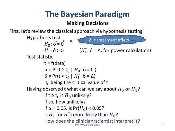
The Bayesian Paradigm δ is treatment effect Phil Woodward 2014 29

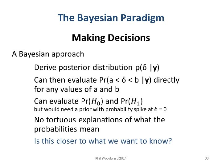
The Bayesian Paradigm Phil Woodward 2014 30

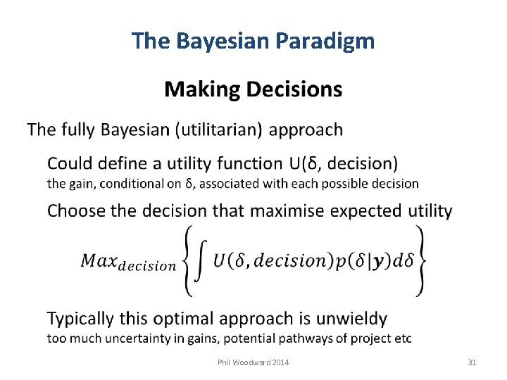
The Bayesian Paradigm Phil Woodward 2014 31

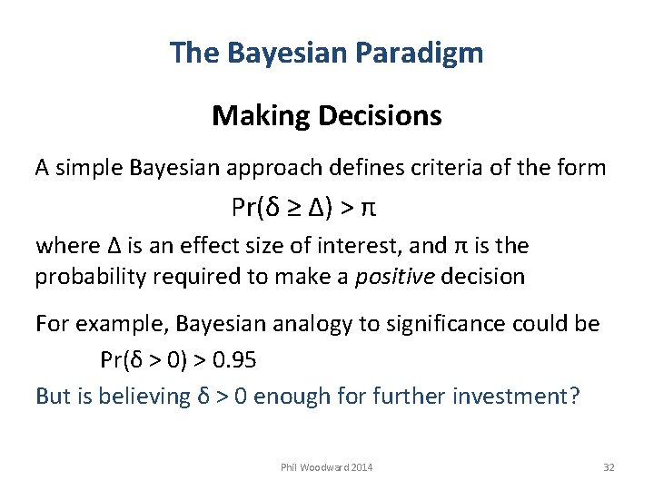
The Bayesian Paradigm Making Decisions A simple Bayesian approach defines criteria of the form Pr(δ ≥ Δ) > π where Δ is an effect size of interest, and π is the probability required to make a positive decision For example, Bayesian analogy to significance could be Pr(δ > 0) > 0. 95 But is believing δ > 0 enough for further investment? Phil Woodward 2014 32

END OF PART 1 intro to Win. BUGS illustrating fixed effect models Phil Woodward 2014 33

Bayesian Model Checking Phil Woodward 2014 34

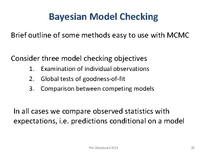
Bayesian Model Checking Brief outline of some methods easy to use with MCMC Consider three model checking objectives 1. Examination of individual observations 2. Global tests of goodness-of-fit 3. Comparison between competing models In all cases we compare observed statistics with expectations, i. e. predictions conditional on a model Phil Woodward 2014 35

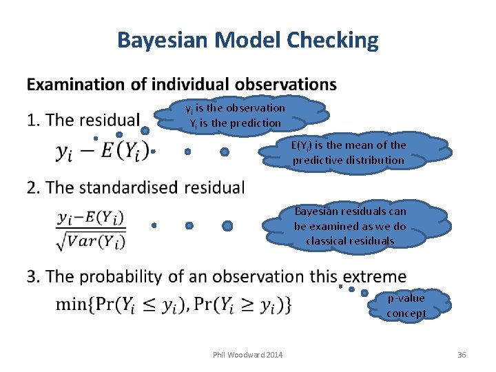
Bayesian Model Checking yi is the observation Yi is the prediction E(Yi) is the mean of the predictive distribution Bayesian residuals can be examined as we do classical residuals p-value concept Phil Woodward 2014 36

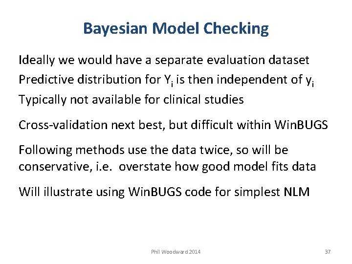
Bayesian Model Checking Ideally we would have a separate evaluation dataset Predictive distribution for Yi is then independent of yi Typically not available for clinical studies Cross-validation next best, but difficult within Win. BUGS Following methods use the data twice, so will be conservative, i. e. overstate how good model fits data Will illustrate using Win. BUGS code for simplest NLM Phil Woodward 2014 37

Bayesian Model Checking (Examination of Individual Observations) { More typically, each Y[i] ### Priors has different mean, mu[i]. mu ~ dnorm(0, 1. 0 E-6) prec ~ dgamma(0. 001, 0. 001) ; sigma <- pow(prec, -0. 5) ### Likelihood for (i in 1: N) { Y[i] ~ dnorm(mu, prec) } each residual has a distribution use the mean as the residual Y. rep[i] is a prediction accounting for uncertainty in parameter values, but not in the type of model assumed ### Model checking for (i in 1: N) { ### Residuals and Standardised Residuals resid[i] <- Y[i] – mu st. resid[i] <- resid[i] / sigma mean of Pr. big[i] estimates the probability a future observation is this big ### Replicate data set & Prob observation is extreme only need both Y. rep[i] ~ dnorm(mu, prec) Pr. big[i] <- step( Y[i] – Y. rep[i] ) when Y. rep[i] could Pr. small[i] <- step( Y. rep[i] – Y[i] ) exactly equal Y[i] } } Phil Woodward 2014 38

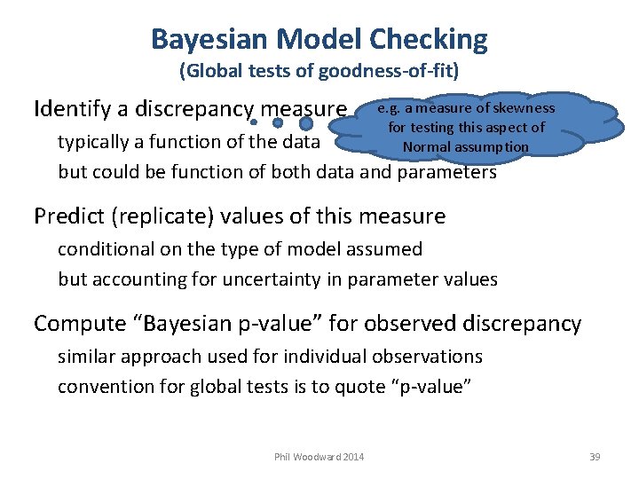
Bayesian Model Checking (Global tests of goodness-of-fit) Identify a discrepancy measure e. g. a measure of skewness for testing this aspect of Normal assumption typically a function of the data but could be function of both data and parameters Predict (replicate) values of this measure conditional on the type of model assumed but accounting for uncertainty in parameter values Compute “Bayesian p-value” for observed discrepancy similar approach used for individual observations convention for global tests is to quote “p-value” Phil Woodward 2014 39

Bayesian Model Checking (Global tests of goodness-of-fit) { … code as before … ### Model checking for (i in 1: N) { ### Residuals and Standardised Residuals resid[i] <- Y[i] – mu st. resid[i] <- resid[i] / sigma m 3[i] <- pow( st. resid[i], 3) ### Replicate data set Y. rep[i] ~ dnorm(mu, prec) resid. rep[i] <- Y. rep[i] – mu[i] st. resid. rep[i] <- resid. rep[i] / sigma m 3. rep[i] <- pow( st. resid. rep[i], 3) } skew <- mean( m 3[] ) skew. rep <- mean( m 3. rep[] ) p. skew. pos <- step( skew. rep – skew ) p. skew. neg <- step( skew – skew. rep ) } p. skew interpreted as for classical p-value, i. e. small is evidence of a discrepancy Phil Woodward 2014 40

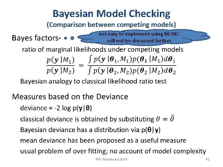
Bayesian Model Checking (Comparison between competing models) Bayes factors not easy to implement using MCMC will not be discussed further ratio of marginal likelihoods under competing models Bayesian analogy to classical likelihood ratio test Phil Woodward 2014 41

Bayesian Model Checking (Comparison between competing models) Deviance Information Criterion (DIC) a Bayesian “information criterion” but not the BIC will not discuss theory, focus on practical interpretation Win. BUGS & SAS can report this for most models DIC is the sum of two separately interpretable quantities DIC = Dbar + p. D Dbar p. D Dhat : the posterior mean of the deviance : the effective number of parameters in the model p. D = Dbar - Dhat : deviance point estimate using posterior mean of θ Phil Woodward 2014 42

Bayesian Model Checking (Comparison between competing models) Deviance Information Criterion (DIC) DIC = Dbar + p. D will differ from the total number of parameters when posterior distributions are correlated typically the case for “random effect parameters” non-orthogonal designs, correlated covariates common for non-linear models p. D will be smaller because some parameters’ effects “overlap” Phil Woodward 2014 43

Bayesian Model Checking (Comparison between competing models) Deviance Information Criterion (DIC) DIC = Dbar + p. D Measures model’s ability to make short-term predictions Smaller values of DIC indicate a better model Rules of thumb for comparing models fitted to the same data DIC difference > 10 is clear evidence of being better DIC difference > 5 (< 10) is still strong evidence There are still some unresolved issues with DIC relatively early days in it use, so use other methods as well Phil Woodward 2014 44

Bayesian Model Checking (practical advice) “All models are wrong, but some are useful” if we keep looking, or have lots of data, we will find lack-of-fit need to assess whether model’s deficiencies matter depends upon the inferences and decisions of interest judge the model on whether it is fit for purpose Sensitivity analyses are useful when uncertain should assess sensitivity to both the likelihood and the prior e. g. replace Normal with t distribution Model expansion may be necessary Bayesian approach particularly good here Informative priors and MCMC allow greater flexibility Phil Woodward 2014 45

Introduction to Bugs. XLA Parallel Group Clinical Study (Analysis of Covariance) Phil Woodward 2014 46

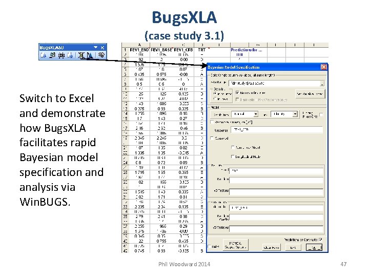
Bugs. XLA (case study 3. 1) Switch to Excel and demonstrate how Bugs. XLA facilitates rapid Bayesian model specification and analysis via Win. BUGS. Phil Woodward 2014 47

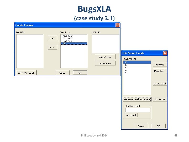
Bugs. XLA (case study 3. 1) Phil Woodward 2014 48

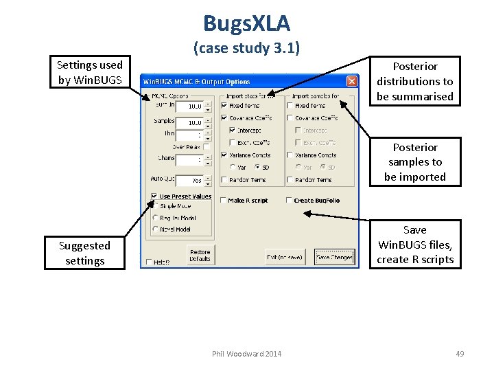
Bugs. XLA Settings used by Win. BUGS (case study 3. 1) Posterior distributions to be summarised Posterior samples to be imported Save Win. BUGS files, create R scripts Suggested settings Phil Woodward 2014 49

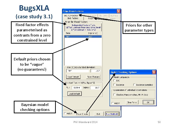
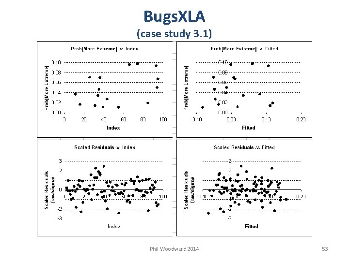
Bugs. XLA (case study 3. 1) Fixed factor effects parameterised as contrasts from a zero constrained level Priors for other parameter types Default priors chosen to be “vague” (no guarantees!) Bayesian model checking options Phil Woodward 2014 50

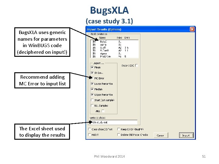
Bugs. XLA (case study 3. 1) Bugs. XLA uses generic names for parameters in Win. BUGS code (deciphered on input!) Recommend adding MC Error to input list The Excel sheet used to display the results Phil Woodward 2014 51

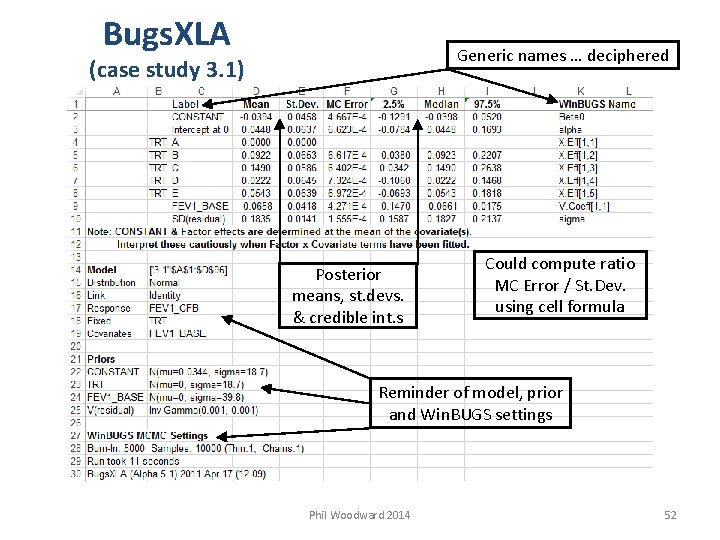
Bugs. XLA Generic names … deciphered (case study 3. 1) Posterior means, st. devs. & credible int. s Could compute ratio MC Error / St. Dev. using cell formula Reminder of model, prior and Win. BUGS settings Phil Woodward 2014 52

Bugs. XLA (case study 3. 1) Phil Woodward 2014 53

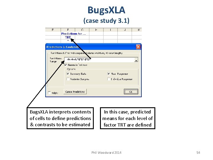
Bugs. XLA (case study 3. 1) Bugs. XLA interprets contents of cells to define predictions & contrasts to be estimated In this case, predicted means for each level of factor TRT are defined Phil Woodward 2014 54

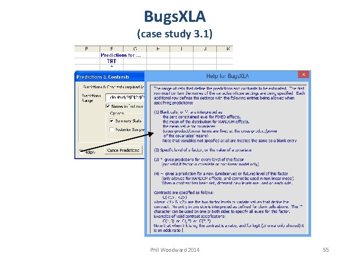
Bugs. XLA (case study 3. 1) Phil Woodward 2014 55

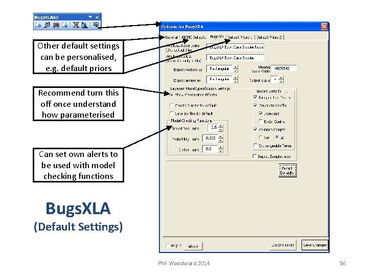
Other default settings can be personalised, e. g. default priors Recommend turn this off once understand how parameterised Can set own alerts to be used with model checking functions Bugs. XLA (Default Settings) Phil Woodward 2014 56

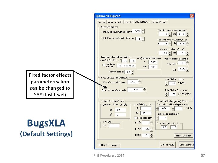
Fixed factor effects parameterisation can be changed to SAS (last level) Bugs. XLA (Default Settings) Phil Woodward 2014 57

Obtaining Prior Distribution Phil Woodward 2014 58

Obtaining Prior Distributions • Brief overview of main approaches* • Further issues in the use of Priors* * based on chapter 5 of Spiegelhalter et al (2004) Phil Woodward 2014 59

Obtaining Prior Distributions • Misconceptions: They are not necessarily – – Prespecified Unique Known Influential • Bayesian analysis – – But prespecification strongly recommended, data must not influence the prior distribution Transforms prior into posterior beliefs Doesn’t produce the posterior distribution Context and audience important Sensitivity to alternative assumptions vital • Prior could differ at design & analysis stage – May want less controversial vague priors in analysis – Design priors usually have to be informative Phil Woodward 2014 60

Obtaining Prior Distributions • Five broad approaches – Elicitation of subjective opinion – Summarising past evidence – Default priors – Robust priors – Estimation using hierarchical models Phil Woodward 2014 61

Obtaining Prior Distributions • Elicitation of subjective opinion – – Most useful when little ‘objective’ evidence Less controversial at the design stage Elicitation should be kept simple & interactive O’Hagan is a strong advocate • Spiegelhalter et al do not recommend – Prefer archetypal views; see Default Priors Phil Woodward 2014 62

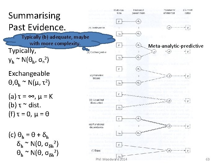
Summarising Past Evidence. Typically (b) adequate, maybe with more complexity. Meta-analytic-predictive Typically, yh ~ N(θh, σh 2) Exchangeable θ, θh ~ N(μ, τ2) (a) τ = ∞, μ = K (b) τ ~ dist. (f) τ = 0, μ = θ (c) θh = θ + δh δh ~ N(0, σδh 2) θh ~ N(θ, σδh 2) Phil Woodward 2014 63

Obtaining Prior Distributions • Default Priors Parameter “big” can be derived via eliciting inferred quantities, e. g. credible differences between study means. – Vague a. k. a. non-informative or reference • Win. BUGS (general advice for ‘simple’ models): – Location parms ~ Normal with huge variance – Lowest level error variance ~ inv-gamma(small, small) – Hierarchical error variances … controverisal sd ~ Uniform(0, big) or ~ Half-Normal(big); big < huge! – Sceptical & Enthusiastic Priors • • Sceptical used to determine when success achieved Enthusiastic used to determine when to stop Sceptical prior centred on 0 with small prob. effect > Δ Enthusiastic prior centred on Δ with small prob. effect < 0 – ‘Lump-and-smear’ Priors • Point mass at the null hypothesis Phil Woodward 2014 Might be appropriate for unprecedented mechanisms in ED stage. 64

Obtaining Prior Distributions • Robust Priors – We always assess model assumptions – Bayesians assess prior assumptions also – Use a ‘community of priors’ • Discrete set • Parametric family • Non-parametric family Perhaps develop a range of priors appropriate in typical case. – Interpretation section recommended in report • Show data affect a range of prior beliefs Phil Woodward 2014 65

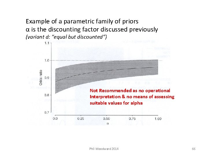
Example of a parametric family of priors α is the discounting factor discussed previously (variant d: “equal but discounted”) Not Recommended as no operational Interpretation & no means of assessing suitable values for alpha Phil Woodward 2014 66

Obtaining Prior Distributions • Hierarchical priors – In simplest case, the same as (b) Exchangeable – ‘Borrow strength’ between studies • counter view: ‘share weakness’ – Three essential ingredients • Exchangeable parameters • Form for random-effects dist. – Typically Normal, although t is perhaps more realistic • Hyperprior for parms of random-effects dist. – sd ~ Uniform(0, Max Credible) or Half-Normal(big) or Half-Cauchy(large) Phil Woodward 2014 67

Obtaining Prior Distributions • Case Study – Dental Pain Studies – Informative prior for placebo mean • Used in the formal analysis – Meta-analytic-predictive approach Phil Woodward 2014 68

Obtaining Prior Distributions (part of table of prior studies considered relevant) TOTPAR[6] Title Characterization of rofecoxib as a cyclooxygenase-2 isoform inhibitor and demonstration of analgesia in the dental pain model Valdecoxib Is More Efficacious Than Rofecoxib in Relieving Pain Associated With Oral Surgery Rofecoxib versus codeine/acetaminophen in postoperative dental pain: a double-blind, randomized, placebo- and active comparator-controlled clinical trial Analgesic Efficacy of Celecoxib in Postoperative Oral Surgery Pain: A Single. Dose, Two-Center, Randomized, Double-Blind, Active- and Placebo. Controlled Study Combination Oxycodone 5 mg/Ibuprofen 400 mg for the Treatment of Postoperative Pain: A Double-Blind, Placebo and Active-Controlled Parallel. Group Study Mean Authors Treatment 3. 01 0. 51 Elliot W. Ehrich et. al Rofecoxib 50 and 500 mg Ibuprofen 400 mg Placebo 3. 01 0. 76 Fricke J. et al. Valdecoxib 40 mg Rofecoxib 50 mg Placebo 3. 4 1. 22 Chang DJ; et al. Rofecoxib 50 mg Codeine/Acetaminophen 60/600 mg Placebo 3. 7 0. 75 Raymond Cheung, et al Celecoxib 400 mg Ibuprofen 400 mg Placebo 4. 2 0. 83 Thomas Van Dyke, et al Oxycodone/Ibuprofen 5 mg/400 mg Ibuprofen 400 mg Oxycodone 5 mg Placebo Phil Woodward 2014 (Placebo Data) SE 69

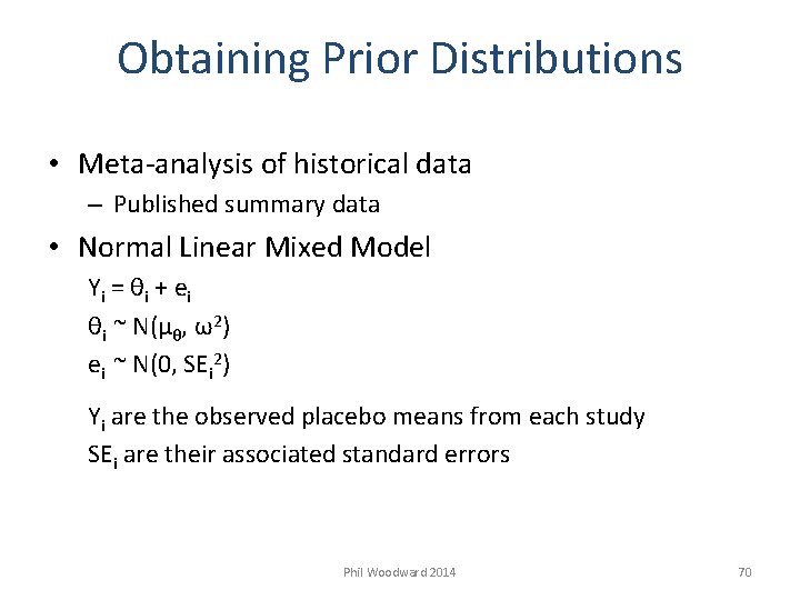
Obtaining Prior Distributions • Meta-analysis of historical data – Published summary data • Normal Linear Mixed Model Yi = θi + ei θi ~ N(µθ, ω2) ei ~ N(0, SEi 2) Yi are the observed placebo means from each study SEi are their associated standard errors Phil Woodward 2014 70

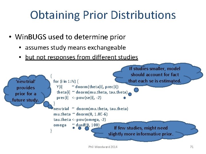
Obtaining Prior Distributions • Win. BUGS used to determine prior • assumes study means exchangeable • but not responses from different studies ‘newtrial’ provides prior for a future study. If studies smaller, model should account for fact that each se is estimated. { for (i in 1: N) { Y[i] ~ dnorm(theta[i], prec[i]) theta[i] ~ dnorm(mu. theta, tau. theta) prec[i] <- pow(se[i], -2) } newtrial ~ dnorm(mu. theta, tau. theta) mu. theta ~ dnorm(0, 1. 0 E-6) tau. theta <- pow(omega, -2) omega ~ dunif(0, 100) If few studies, might need } slightly more informative prior. Phil Woodward 2014 71

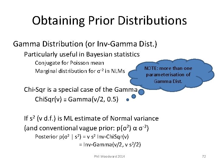
Obtaining Prior Distributions Gamma Distribution (or Inv-Gamma Dist. ) Particularly useful in Bayesian statistics Conjugate for Poisson mean Marginal distribution for σ-2 in NLMs NOTE: more than one parameterisation of Gamma Dist. Chi-Sqr is a special case of the Gamma Chi. Sqr(v) ≡ Gamma(v/2, 0. 5) If s 2 (v d. f. ) is ML estimate of Normal variance (and conventional vague prior: p(σ2) α σ-2) Posterior p(σ2 | s 2) = v s 2 Inv-Chi. Sqr(v) = Inv-Gamma(v/2, v s 2/2) Phil Woodward 2014 72

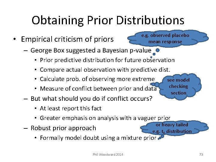
Obtaining Prior Distributions • Empirical criticism of priors e. g. observed placebo mean response – George Box suggested a Bayesian p-value • • Prior predictive distribution for future observation Compare actual observation with predictive dist. Calculate prob. of observing more extreme see model checking Measure of conflict between prior and data – But what should you do if conflict occurs? section • At least report this fact • Greater emphasis on analysis with a vaguer prior – Robust prior approach or heavy tailed e. g. t 4 distribution • Formally model doubt using a mixture prior Phil Woodward 2014 73

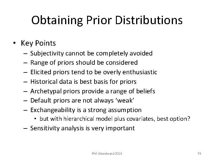
Obtaining Prior Distributions • Key Points – – – – Subjectivity cannot be completely avoided Range of priors should be considered Elicited priors tend to be overly enthusiastic Historical data is best basis for priors Archetypal priors provide a range of beliefs Default priors are not always ‘weak’ Exchangeability is a strong assumption • but with hierarchical model plus covariates, best option? – Sensitivity analysis is very important Phil Woodward 2014 74

Bugs. XLA Deriving and using informative prior distributions Phil Woodward 2014 75

Bugs. XLA (case study 5. 3, details not covered in this course) Predict placebo mean response in a future study Bugs. XLA can model study level summary statistics (d. f. optional) Typically, model is much simpler than this, e. g. placebo data only, no study level covariates, so only random STUDY factor in model Phil Woodward 2014 76

Bugs. XLA (using informative prior distributions) Back to Case Study 3. 1 Will assume have derived informative priors for: Placebo mean response Normal with mean 0 and standard deviation 0. 04 Residual variance Scaled Chi-Square with s 2 = 0. 026 and df = 44 Switch back to Excel and show to use this in Bugs. XLA Phil Woodward 2014 77

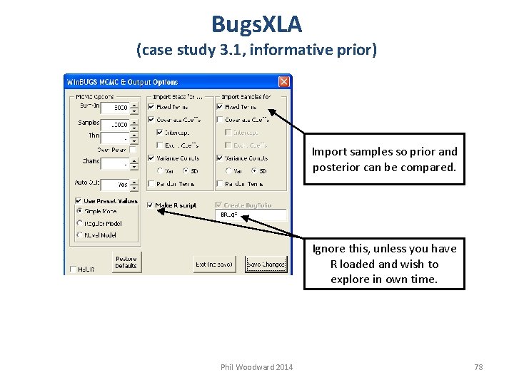
Bugs. XLA (case study 3. 1, informative prior) Import samples so prior and posterior can be compared. Ignore this, unless you have R loaded and wish to explore in own time. Phil Woodward 2014 78

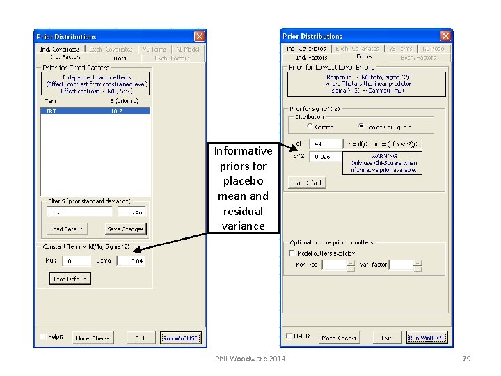
Informative priors for placebo mean and residual variance Phil Woodward 2014 79

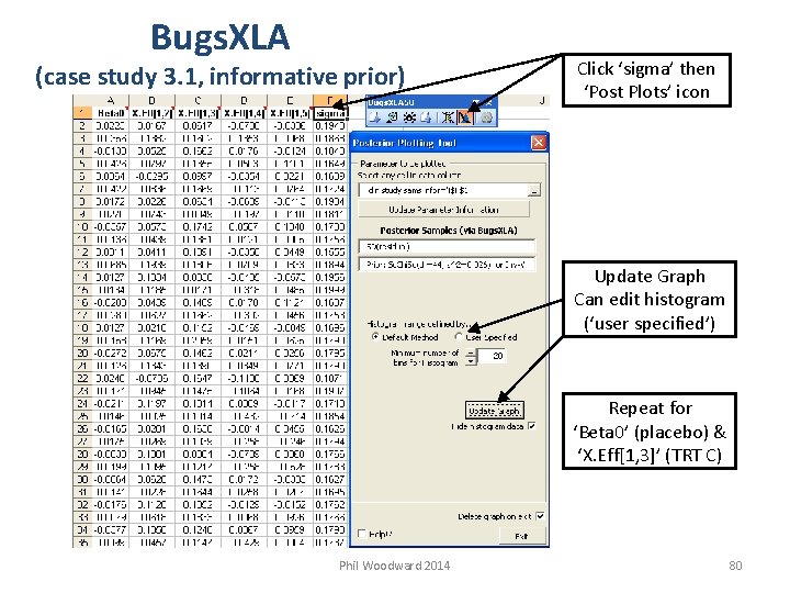
Bugs. XLA (case study 3. 1, informative prior) Click ‘sigma’ then ‘Post Plots’ icon Update Graph Can edit histogram (‘user specified’) Repeat for ‘Beta 0’ (placebo) & ‘X. Eff[1, 3]’ (TRT C) Phil Woodward 2014 80

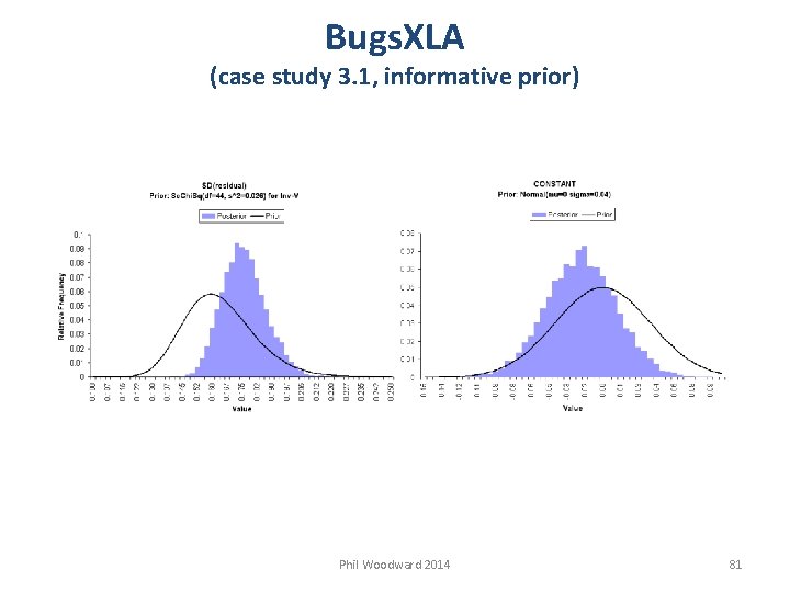
Bugs. XLA (case study 3. 1, informative prior) Phil Woodward 2014 81

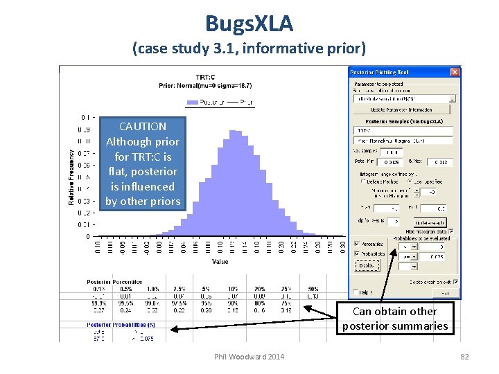
Bugs. XLA (case study 3. 1, informative prior) CAUTION Although prior for TRT: C is flat, posterior is influenced by other priors Can obtain other posterior summaries Phil Woodward 2014 82

Bayesian Study Design Phil Woodward 2014 83

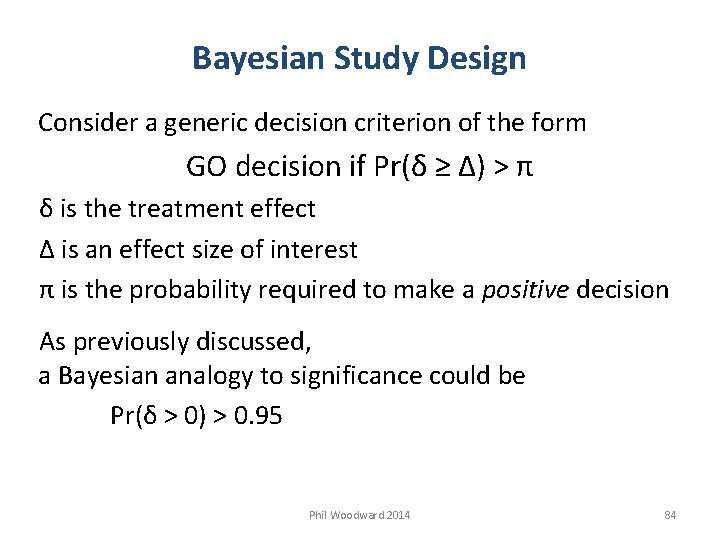
Bayesian Study Design Consider a generic decision criterion of the form GO decision if Pr(δ ≥ Δ) > π δ is the treatment effect Δ is an effect size of interest π is the probability required to make a positive decision As previously discussed, a Bayesian analogy to significance could be Pr(δ > 0) > 0. 95 Phil Woodward 2014 84

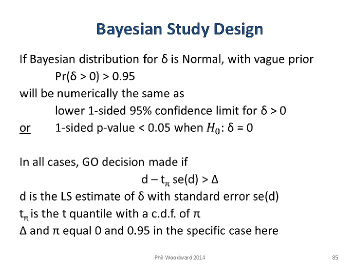
Bayesian Study Design Phil Woodward 2014 85

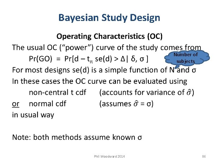
Bayesian Study Design Number of subjects Phil Woodward 2014 86

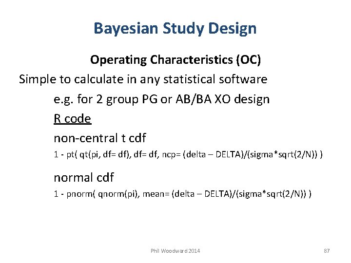
Bayesian Study Design Operating Characteristics (OC) Simple to calculate in any statistical software e. g. for 2 group PG or AB/BA XO design R code non-central t cdf 1 - pt( qt(pi, df= df), df= df, ncp= (delta – DELTA)/(sigma*sqrt(2/N)) ) normal cdf 1 - pnorm( qnorm(pi), mean= (delta – DELTA)/(sigma*sqrt(2/N)) ) Phil Woodward 2014 87

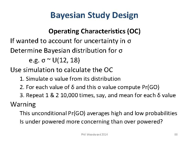
Bayesian Study Design Operating Characteristics (OC) If wanted to account for uncertainty in σ Determine Bayesian distribution for σ e. g. σ ~ U(12, 18) Use simulation to calculate the OC 1. Simulate σ value from its distribution 2. For each value of δ and this σ value compute Pr(GO) 3. Repeat 1 & 2 10, 000 times, say, and mean for each δ value Warning This unconditional Pr(GO) averages high and low probabilities Is under powered more concerning than over powered? Phil Woodward 2014 88

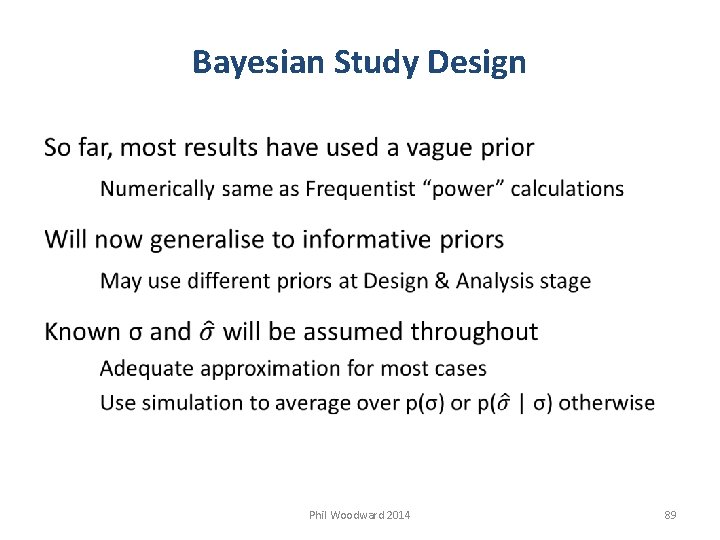
Bayesian Study Design Phil Woodward 2014 89

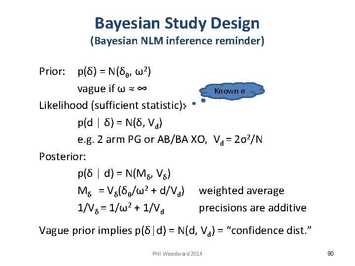
Bayesian Study Design (Bayesian NLM inference reminder) Prior: p(δ) = N(δ 0, ω2) vague if ω ≈ ∞ Known σ Likelihood (sufficient statistic): p(d | δ) = N(δ, Vd) e. g. 2 arm PG or AB/BA XO, Vd = 2σ2/N Posterior: p(δ | d) = N(Mδ, Vδ) Mδ = Vδ(δ 0/ω2 + d/Vd) weighted average 1/Vδ = 1/ω2 + 1/Vd precisions are additive Vague prior implies p(δ|d) = N(d, Vd) = “confidence dist. ” Phil Woodward 2014 90

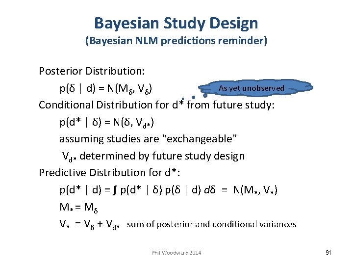
Bayesian Study Design (Bayesian NLM predictions reminder) Posterior Distribution: As yet unobserved p(δ | d) = N(Mδ, Vδ) Conditional Distribution for d* from future study: p(d* | δ) = N(δ, Vd*) assuming studies are “exchangeable” Vd* determined by future study design Predictive Distribution for d*: p(d* | d) = ∫ p(d* | δ) p(δ | d) dδ = N(M*, V*) M* = Mδ V* = Vδ + Vd* sum of posterior and conditional variances Phil Woodward 2014 91

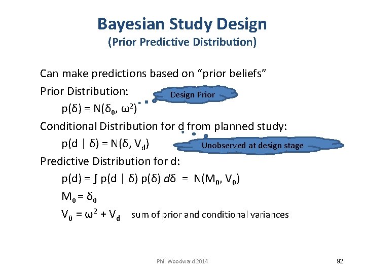
Bayesian Study Design (Prior Predictive Distribution) Can make predictions based on “prior beliefs” Prior Distribution: Design Prior p(δ) = N(δ 0, ω2) Conditional Distribution for d from planned study: p(d | δ) = N(δ, Vd) Unobserved at design stage Predictive Distribution for d: p(d) = ∫ p(d | δ) p(δ) dδ = N(M 0, V 0) M 0 = δ 0 V 0 = ω2 + Vd sum of prior and conditional variances Phil Woodward 2014 92

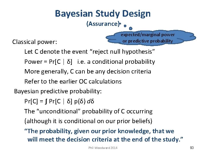
Bayesian Study Design (Assurance) expected/marginal power or predictive probability Classical power: Let C denote the event “reject null hypothesis” Power = Pr[C | δ] i. e. a conditional probability More generally, C can be any decision criteria Refer to the earlier OC calculations Bayesian predictive probability: Pr[C] = ∫ Pr[C | δ] p(δ) dδ The “unconditional” probability of C occurring (although it is conditional on our prior beliefs) “The probability, given our prior knowledge, that we will meet the decision criteria at the end of the study. ” Phil Woodward 2014 93

Bayesian Study Design (Assurance) Consider original GO decision Pr[C | d] = Pr[d – tπ se(d) > Δ] with vague Analysis Prior p(d) = N(δ 0, ω2 + Vd) prior predictive distribution with informative Design Prior Pr[C] = Pr[ N(δ 0, ω2 + Vd) > tπ se(d) + Δ] Pr[C] = Φ[δ 0 – tπ se(d) – Δ) / (ω2 + Vd)½] where Φ[. ] is the standard Normal cdf What if vague Design Prior, i. e. ω very large? Phil Woodward 2014 94

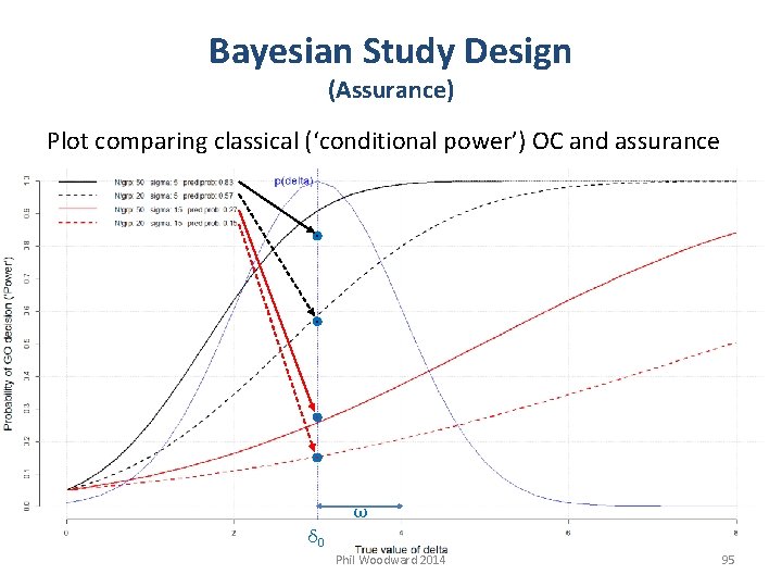
Bayesian Study Design (Assurance) Plot comparing classical (‘conditional power’) OC and assurance ω δ 0 Phil Woodward 2014 95

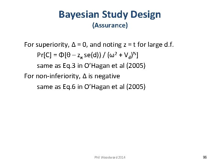
Bayesian Study Design (Assurance) For superiority, Δ = 0, and noting z = t for large d. f. Pr[C] = Φ[θ – zπ se(d)) / (ω2 + Vd)½] same as Eq. 3 in O’Hagan et al (2005) For non-inferiority, Δ is negative same as Eq. 6 in O’Hagan et al (2005) Phil Woodward 2014 96

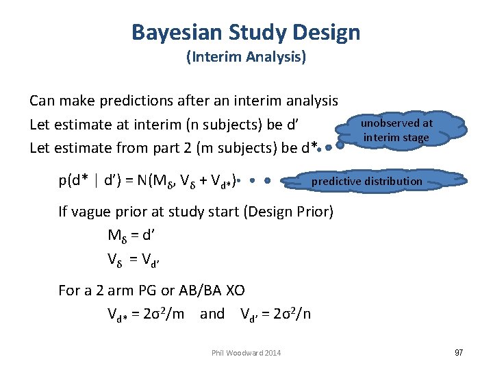
Bayesian Study Design (Interim Analysis) Can make predictions after an interim analysis Let estimate at interim (n subjects) be d’ Let estimate from part 2 (m subjects) be d* p(d* | d’) = N(Mδ, Vδ + Vd*) unobserved at interim stage predictive distribution If vague prior at study start (Design Prior) Mδ = d’ Vδ = Vd’ For a 2 arm PG or AB/BA XO Vd* = 2σ2/m and Vd’ = 2σ2/n Phil Woodward 2014 97

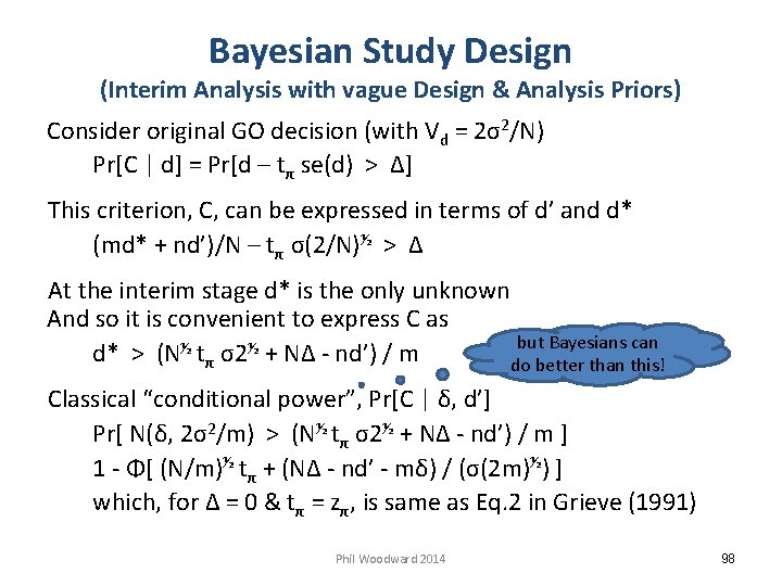
Bayesian Study Design (Interim Analysis with vague Design & Analysis Priors) Consider original GO decision (with Vd = 2σ2/N) Pr[C | d] = Pr[d – tπ se(d) > Δ] This criterion, C, can be expressed in terms of d’ and d* (md* + nd’)/N – tπ σ(2/N)½ > Δ At the interim stage d* is the only unknown And so it is convenient to express C as but Bayesians can d* > (N½ tπ σ2½ + NΔ - nd’) / m do better than this! Classical “conditional power”, Pr[C | δ, d’] Pr[ N(δ, 2σ2/m) > (N½ tπ σ2½ + NΔ - nd’) / m ] 1 - Φ[ (N/m)½ tπ + (NΔ - nd’ - mδ) / (σ(2 m)½) ] which, for Δ = 0 & tπ = zπ, is same as Eq. 2 in Grieve (1991) Phil Woodward 2014 98

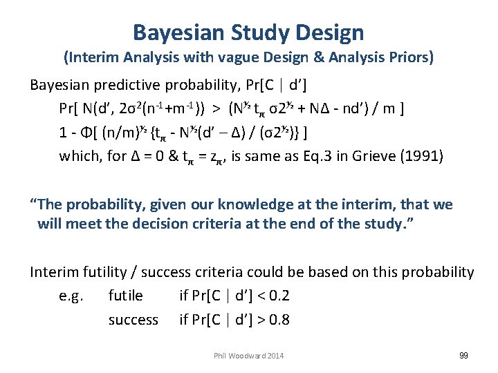
Bayesian Study Design (Interim Analysis with vague Design & Analysis Priors) Bayesian predictive probability, Pr[C | d’] Pr[ N(d’, 2σ2(n-1+m-1)) > (N½ tπ σ2½ + NΔ - nd’) / m ] 1 - Φ[ (n/m)½ {tπ - N½(d’ – Δ) / (σ2½)} ] which, for Δ = 0 & tπ = zπ, is same as Eq. 3 in Grieve (1991) “The probability, given our knowledge at the interim, that we will meet the decision criteria at the end of the study. ” Interim futility / success criteria could be based on this probability e. g. futile if Pr[C | d’] < 0. 2 success if Pr[C | d’] > 0. 8 Phil Woodward 2014 99

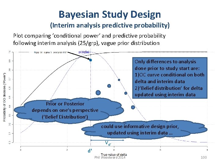
Bayesian Study Design (Interim analysis predictive probability) Plot comparing ‘conditional power’ and predictive probability following interim analysis (25/grp), vague prior distribution Only differences to analysis done prior to study start are: 1)OC curve conditional on both delta and interim data 2)‘Belief distribution’ for delta updated using interim data Prior or Posterior depends on one’s perspective (‘Belief Distribution’) could use informative design prior, updated using interim data … Vd’ d' Phil Woodward 2014 100

Bayesian Study Design (Interim Analysis with informative Design Prior) If we allow an informative design prior at study start refer back to p(δ) = N(δ 0, ω2) Bayesian NLM reminders p(d* | d’) = N(Mδ, Vδ + 2σ2/m) Mδ = Vδ(δ 0/ω2 + d’n/(2σ2)) 1/Vδ = 1/ω2 + n/(2σ2) Bayesian predictive probability, Pr[C | d’] Pr[ N(Mδ, Vδ + 2σ2/m) > (N½ tπ σ2½ + NΔ - nd’) / m ] 1 - Φ[(N½ tπ σ2½ - nd’ - m. Mδ + NΔ) / (m(Vδ + 2σ2/m)½) still with vague analysis prior Phil Woodward 2014 101

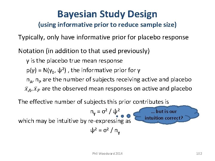
Bayesian Study Design (using informative prior to reduce sample size) Typically, only have informative prior for placebo response Notation (in addition to that used previously) γ is the placebo true mean response p(γ) = N(γ 0, ψ2) , the informative prior for γ n. A, n. P are the number of subjects receiving active and placebo The effective number of subjects this prior contributes is … but is our nγ = σ2 / ψ2 intuition correct? which may be intuitive by re-expressing as ψ2 = σ2 / nγ Phil Woodward 2014 102

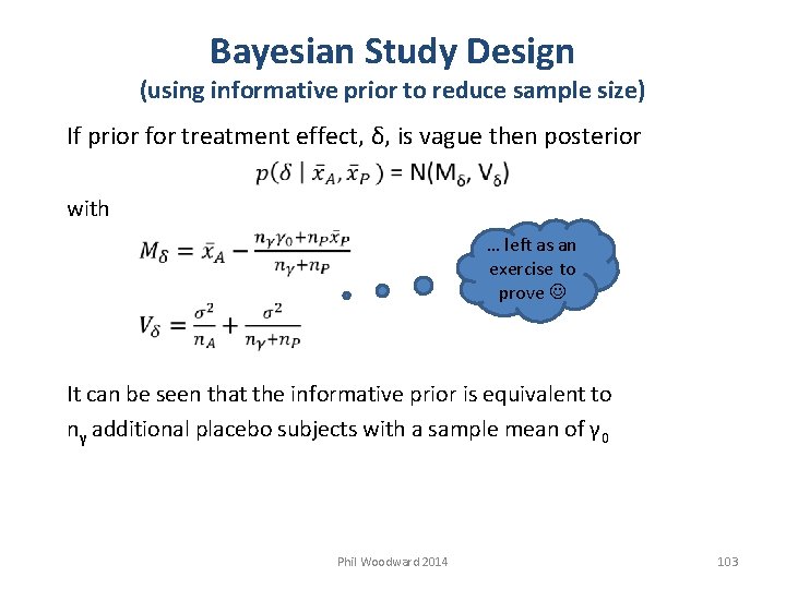
Bayesian Study Design (using informative prior to reduce sample size) If prior for treatment effect, δ, is vague then posterior with … left as an exercise to prove It can be seen that the informative prior is equivalent to nγ additional placebo subjects with a sample mean of γ 0 Phil Woodward 2014 103

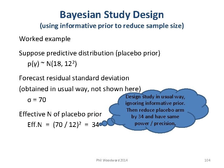
Bayesian Study Design (using informative prior to reduce sample size) Worked example Suppose predictive distribution (placebo prior) p(γ) ~ N(18, 122) Forecast residual standard deviation (obtained in usual way, not shown here) Design study in usual way, σ = 70 ignoring informative prior. Effective N of placebo prior Eff. N = (70 / 12)2 = 34 Then reduce placebo arm by 34 and have same power / precision. Phil Woodward 2014 104

Bayesian Study Design (using informative prior to reduce sample size) Unless no doubts at all, use Robust Prior i. e. a mixture of informative and vague prior distributions p(placebo mean) ~ 0. 9 x N(18, 122) + 0. 1 x N(18, 1202) Represents 10% chance meta-data not exchangeable in which case, will effectively revert to vague prior (can also be thought of as heavy tailed distribution) Also compute Bayesian p-value of data-prior compatibility Pr( “> observed mean” | prior ~ N(18, 122) ) Note: predictive dist. for obs. mean ~ N(18, 122 + σ2 /n. P) Phil Woodward 2014 105

Bayesian Emax Model dose/concentration response model Phil Woodward 2014 106

Bayesian Emax Model Emax model is often used for dose response data even more common for concentration response data in biological (non-clinical) context known as the logistic or sigmoidal curve More generally, could be used to model a monotonic relationship between response and covariate initially the response changes very slowly with the covariate then the response changes much more rapidly finally the response slows again as a plateau is reached Phil Woodward 2014 107

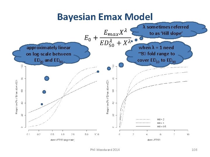
Bayesian Emax Model λ sometimes referred to as ‘Hill slope’ when λ = 1 need ~80 fold range to cover ED 10 to ED 90 approximately linear on log-scale between ED 20 and ED 80 Phil Woodward 2014 108

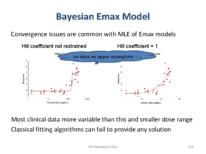
Bayesian Emax Model Convergence issues are common with MLE of Emax models Hill coefficient not restrained Hill coefficient = 1 no data on upper asymptote Most clinical data more variable than this and smaller dose range Classical fitting algorithms can fail to provide any solution Phil Woodward 2014 109

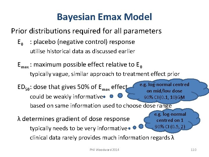
Bayesian Emax Model Prior distributions required for all parameters E 0 : placebo (negative control) response utilise historical data as discussed earlier Emax : maximum possible effect relative to E 0 typically vague, similar approach to treatment effect prior ED 50: dose that gives 50% of Emax effect e. g. log-normal centred on mid/low dose 90% CI (0. 1, 10)GM could be weakly informative based on same information used to choose dose range λ determines gradient of dose response e. g. log-normal centred on 1 90% CI (0. 5, 2) typically needs to be very informative clinical data rarely provides much information regards λ Phil Woodward 2014 110

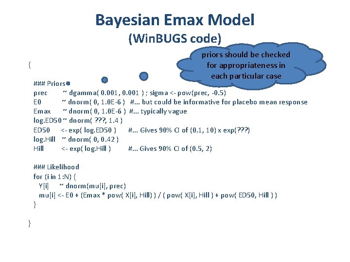
Bayesian Emax Model (Win. BUGS code) { priors should be checked for appropriateness in each particular case ### Priors prec ~ dgamma( 0. 001, 0. 001 ) ; sigma <- pow(prec, -0. 5) E 0 ~ dnorm( 0, 1. 0 E-6 ) #. . . but could be informative for placebo mean response Emax ~ dnorm( 0, 1. 0 E-6 ) #. . . typically vague log. ED 50 ~ dnorm( ? ? ? , 1. 4 ) ED 50 <- exp( log. ED 50 ) #. . . Gives 90% CI of (0. 1, 10) x exp(? ? ? ) log. Hill ~ dnorm( 0, 0. 42 ) Hill <- exp( log. Hill ) #. . . Gives 90% CI of (0. 5, 2) ### Likelihood for (i in 1: N) { Y[i] ~ dnorm(mu[i], prec) mu[i] <- E 0 + (Emax * pow( X[i], Hill) ) / ( pow( X[i], Hill ) + pow( ED 50, Hill ) ) } }

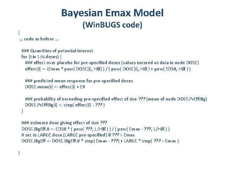
Bayesian Emax Model { … code as before … (Win. BUGS code) ### Quantities of potential interest for (i in 1: N. doses) { ### effect over placebo for pre-specified doses (values entered as data in node DOSE) effect[i] <- (Emax * pow( DOSE[i], Hill) ) / ( pow( DOSE[i], Hill ) + pow( ED 50, Hill ) ) ### predicted mean response for pre-specified doses DOSE. mean[i] <- effect[i] + E 0 ### probability of exceeding pre-specified effect of size ? ? ? (mean of node DOSE. Pr. Eff. Big) DOSE. Pr. Eff. Big[i] <- step( effect[i] - ? ? ? ) } ### estimate dose giving effect of size ? ? ? DOSE. Big. Eff. 0 <- ED 50 * ( pow( ? ? ? , 1/Hill ) ) / ( pow( Emax - ? ? ? , 1/Hill ) ) # set to LARGE dose (LARGE pre-specified) if ? ? ? > Emax DOSE. Big. Eff <- DOSE. Big. Eff. 0 * step( Emax - ? ? ? ) + LARGE * step( ? ? ? – Emax ) }

Bugs. XLA Emax models Pharmacology Biomarker Experiment Phil Woodward 2014 113

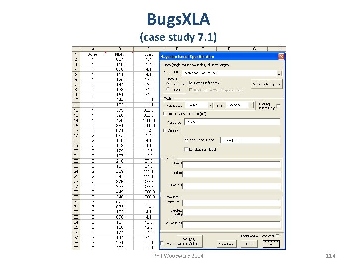
Bugs. XLA (case study 7. 1) Phil Woodward 2014 114

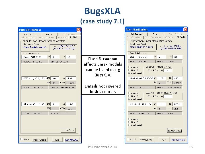
Bugs. XLA (case study 7. 1) Fixed & random effects Emax models can be fitted using Bugs. XLA. Details not covered in this course. Phil Woodward 2014 115

References Bolstad, W. M. (2007). Introduction to Bayesian Statistics. 2 nd Edition. John Wiley & Sons, New York. Gelman, A. , Carlin, J. B. , Stern, H. S. and Rubin, D. B. (2004). Bayesian Data Analysis. 2 nd Edition. Chapman & Hall/CRC. (3 rd Edition now available). Grieve, A. (1991). Predictive probability in clinical trials. Biometrics, 47, 323 -330 Lee, P. M. (2004). Bayesian Statistics: An Introduction. 3 rd Edition. Hodder Arnold, London, U. K. Neuenschwander, B. , Capkun-Niggli, G. , Branson, M. and Spiegelhalter, D. J. (2010). Summarizing historical information on controls in clinical trials. Clinical Trials; 7: 5 -18 Ntzoufras, I. (2009). Bayesian Modeling Using Win. BUGS. John Wiley & Sons, Hoboken, NJ. O’Hagan, A. , Stevens, J. and Campbell, M. (2005). Assurance in clinical trial design. Pharmaceut. Statist. 4, 187201 Spiegelhalter, D. , Abrams, K. and Myles, J. (2004). Bayesian Approaches to Clinical Trials and Health-Care Evaluation. John Wiley & Sons, New York. Woodward, P. (2012). Bayesian Analysis Made Simple. An Excel GUI for Win. BUGS. Chapman & Hall/CRC. Phil Woodward 2014 116