Applications of the Basic Equations Kinematics and Dynamics

Applications of the Basic Equations • Outline of this lecture packet… • • Basic equations in isobaric coordinates Balanced flow Trajectories and streamlines The thermal wind Vertical motion Computer weather model considerations Surface pressure tendency

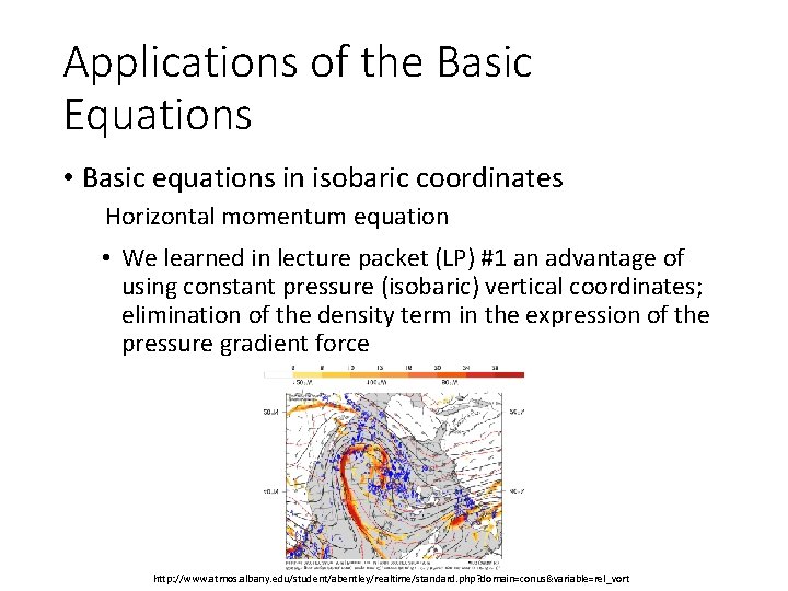
Applications of the Basic Equations • Basic equations in isobaric coordinates Horizontal momentum equation • We learned in lecture packet (LP) #1 an advantage of using constant pressure (isobaric) vertical coordinates; elimination of the density term in the expression of the pressure gradient force http: //www. atmos. albany. edu/student/abentley/realtime/standard. php? domain=conus&variable=rel_vort

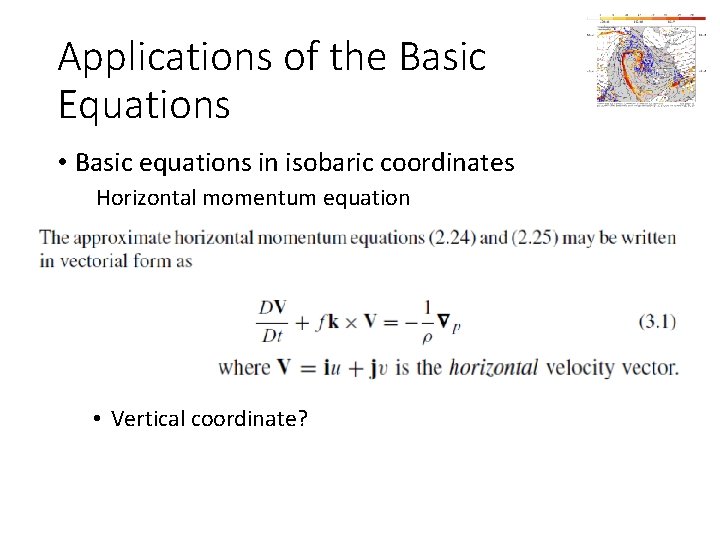
Applications of the Basic Equations • Basic equations in isobaric coordinates Horizontal momentum equation • Vertical coordinate?

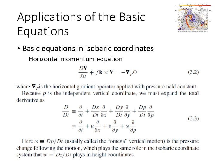
Applications of the Basic Equations • Basic equations in isobaric coordinates Horizontal momentum equation

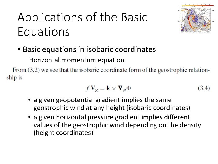
Applications of the Basic Equations • Basic equations in isobaric coordinates Horizontal momentum equation • a given geopotential gradient implies the same geostrophic wind at any height (isobaric coordinates) • a given horizontal pressure gradient implies different values of the geostrophic wind depending on the density (height coordinates)

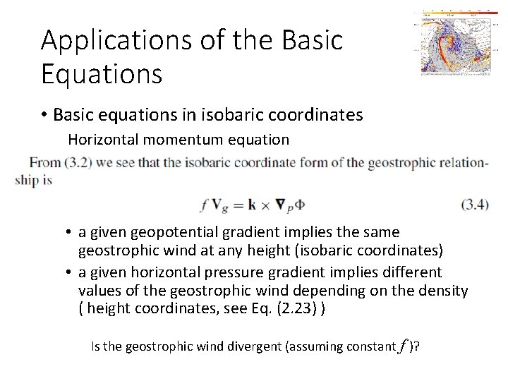
Applications of the Basic Equations • Basic equations in isobaric coordinates Horizontal momentum equation • a given geopotential gradient implies the same geostrophic wind at any height (isobaric coordinates) • a given horizontal pressure gradient implies different values of the geostrophic wind depending on the density ( height coordinates, see Eq. (2. 23) ) Is the geostrophic wind divergent (assuming constant f )?

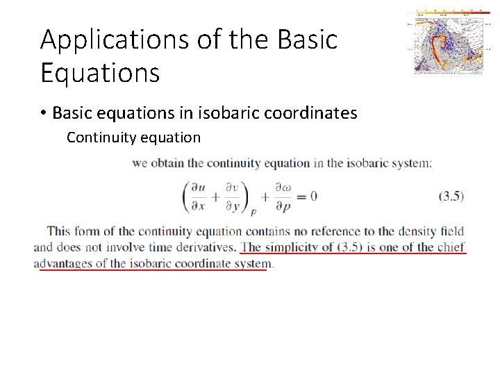
Applications of the Basic Equations • Basic equations in isobaric coordinates Continuity equation

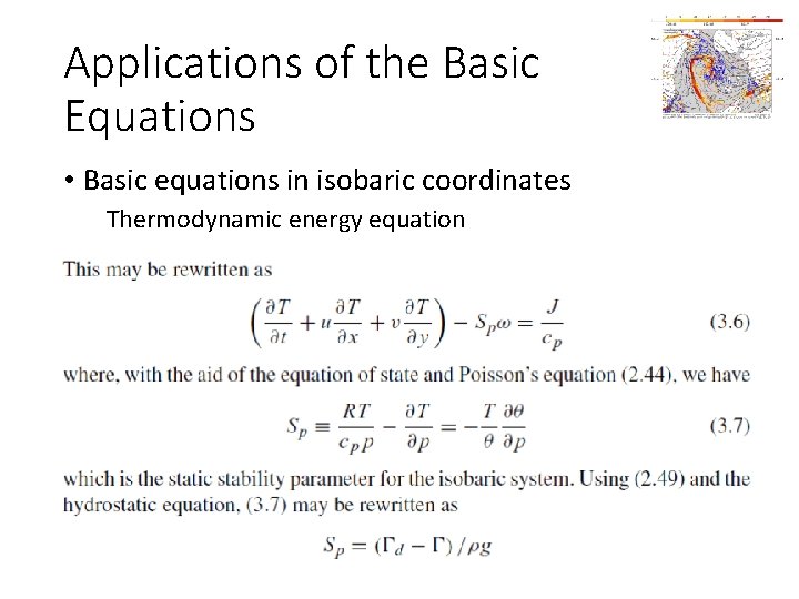
Applications of the Basic Equations • Basic equations in isobaric coordinates Thermodynamic energy equation

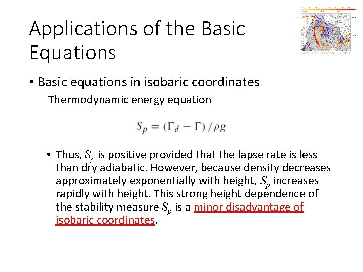
Applications of the Basic Equations • Basic equations in isobaric coordinates Thermodynamic energy equation • Thus, Sp is positive provided that the lapse rate is less than dry adiabatic. However, because density decreases approximately exponentially with height, Sp increases rapidly with height. This strong height dependence of the stability measure Sp is a minor disadvantage of isobaric coordinates.

Applications of the Basic Equations • Balanced flow Introduction • To better visualize approximate atmospheric balances observed on the synoptic scale, we assume [1] steady state (time independent) flow [2] no vertical velocity https%3 A%2 F%2 Fwww. amizonasci. com%2 Fproduct%2 Fcompact-balance-series-readability-0 -1 -to-0 -01 g%2 F&psig=AOv. Vaw 0 JYf. Qfb 4 n 4 h. CCRcx. Kj 2 x. Ww&ust=1577629846547641

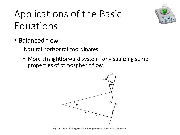
Applications of the Basic Equations • Balanced flow Natural horizontal coordinates • More straightforward system for visualizing some properties of atmospheric flow

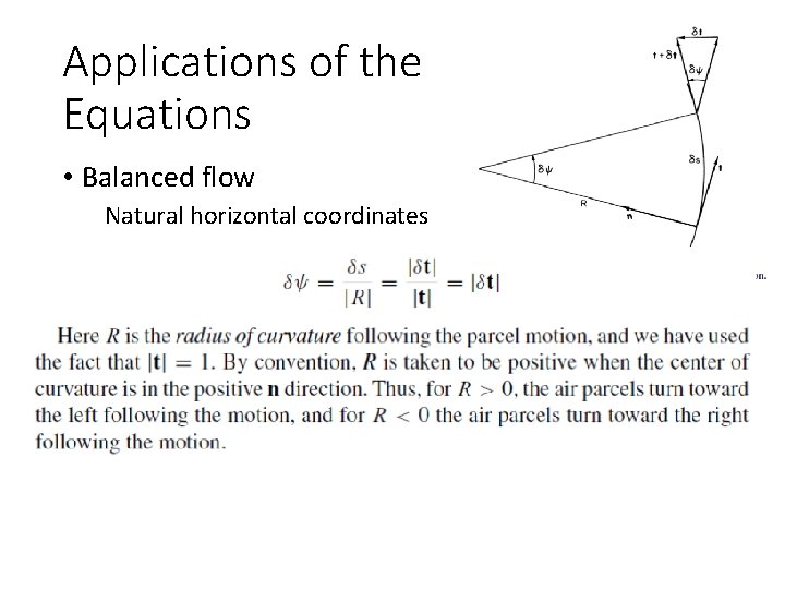
Applications of the Basic Equations • Balanced flow Natural horizontal coordinates

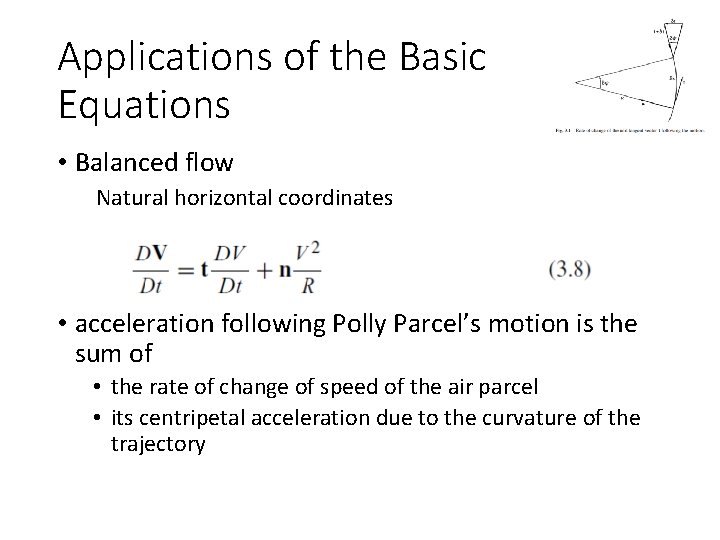
Applications of the Basic Equations • Balanced flow Natural horizontal coordinates • acceleration following Polly Parcel’s motion is the sum of • the rate of change of speed of the air parcel • its centripetal acceleration due to the curvature of the trajectory

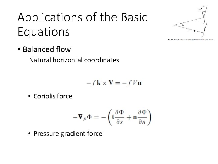
Applications of the Basic Equations • Balanced flow Natural horizontal coordinates • Coriolis force • Pressure gradient force

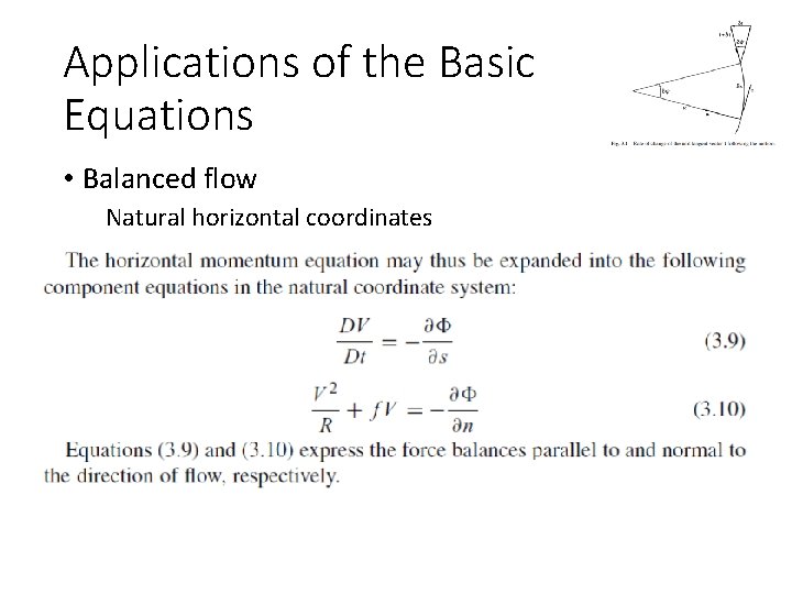
Applications of the Basic Equations • Balanced flow Natural horizontal coordinates

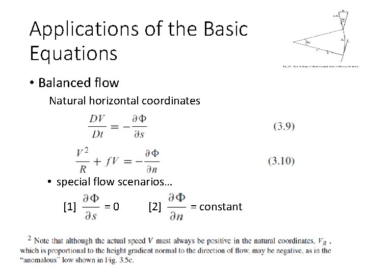
Applications of the Basic Equations • Balanced flow Natural horizontal coordinates • special flow scenarios… [1] =0 [2] = constant

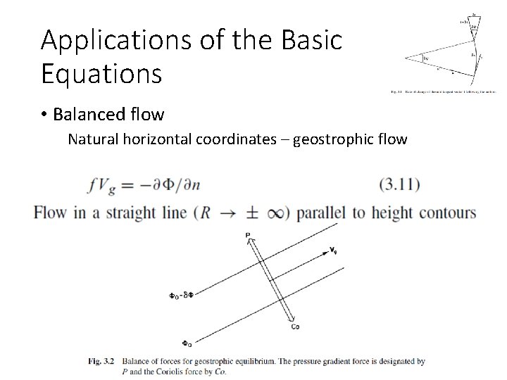
Applications of the Basic Equations • Balanced flow Natural horizontal coordinates – geostrophic flow

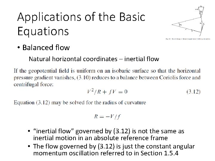
Applications of the Basic Equations • Balanced flow Natural horizontal coordinates – inertial flow • “inertial flow” governed by (3. 12) is not the same as inertial motion in an absolute reference frame • The flow governed by (3. 12) is just the constant angular momentum oscillation referred to in Section 1. 5. 4

Applications of the Basic Equations • Balanced flow Natural horizontal coordinates – inertial flow • In the atmosphere, motions are nearly always generated and maintained by pressure gradient forces; the conditions of uniform pressure required for pure inertial flow rarely exist.

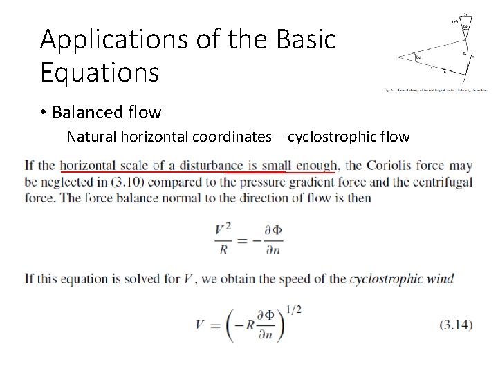
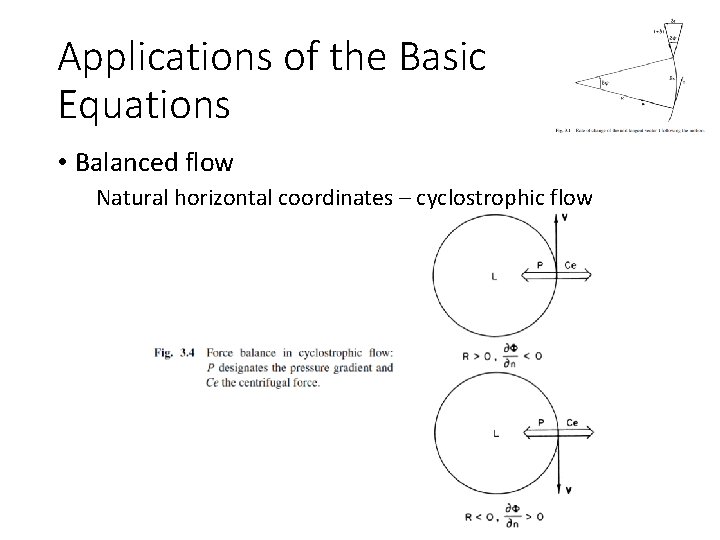
Applications of the Basic Equations • Balanced flow Natural horizontal coordinates – cyclostrophic flow

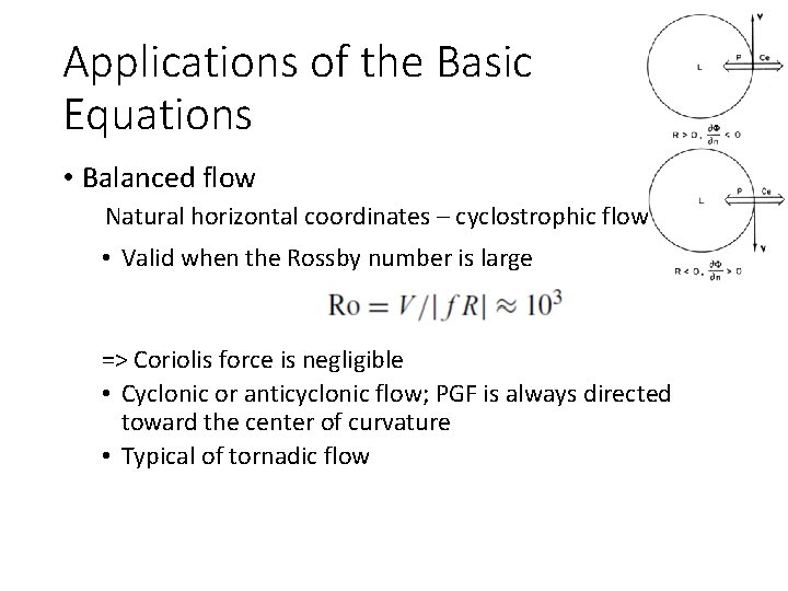
Applications of the Basic Equations • Balanced flow Natural horizontal coordinates – cyclostrophic flow • Valid when the Rossby number is large => Coriolis force is negligible • Cyclonic or anticyclonic flow; PGF is always directed toward the center of curvature • Typical of tornadic flow

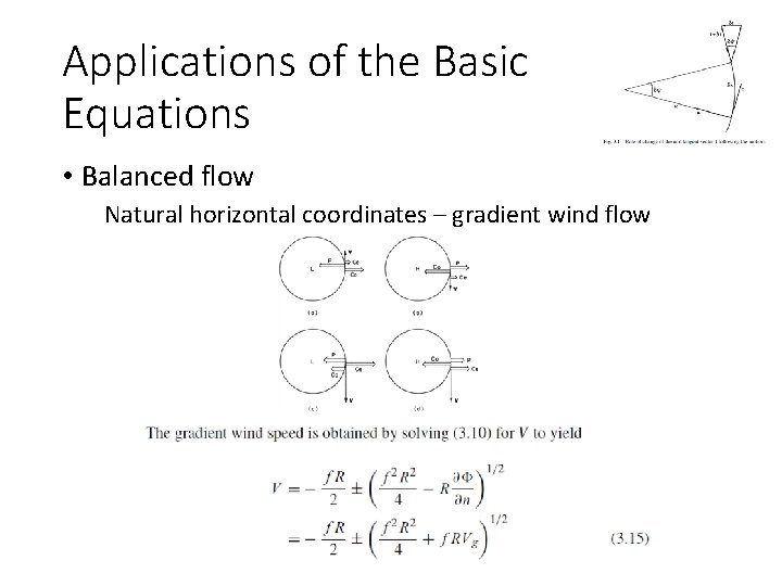
Applications of the Basic Equations • Balanced flow Natural horizontal coordinates – gradient wind flow

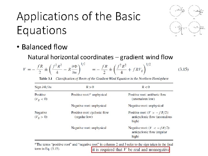
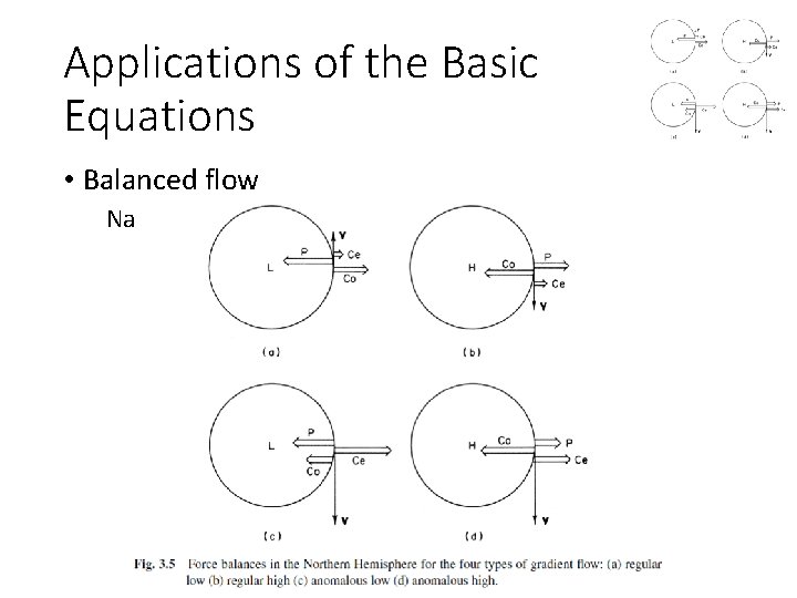
Applications of the Basic Equations • Balanced flow Natural horizontal coordinates – gradient wind flow • a three-way balance among the Coriolis force, the centrifugal force, and the horizontal pressure gradient force • can exist only under very special circumstances • it is always possible, however, to define a gradient wind, which at any point is just the wind component parallel to the height contours that satisfies (3. 10) • because (3. 10) takes into account the centrifugal force due to the curvature of parcel trajectories, the gradient wind is often a better approximation to the actual wind than the geostrophic wind

Applications of the Basic Equations • Balanced flow Natural horizontal coordinates – gradient wind flow

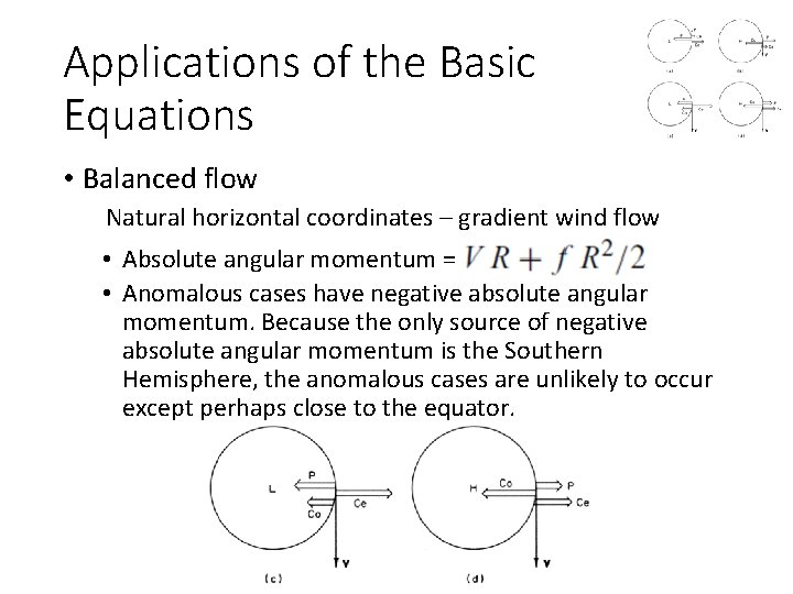
Applications of the Basic Equations • Balanced flow Natural horizontal coordinates – gradient wind flow • Absolute angular momentum = • Anomalous cases have negative absolute angular momentum. Because the only source of negative absolute angular momentum is the Southern Hemisphere, the anomalous cases are unlikely to occur except perhaps close to the equator.

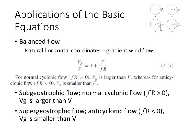
Applications of the Basic Equations • Balanced flow Natural horizontal coordinates – gradient wind flow • Subgeostrophic flow; normal cyclonic flow ( f R > 0), Vg is larger than V • Supergeostrophic flow; anticyclonic flow ( f R < 0), Vg is smaller than V

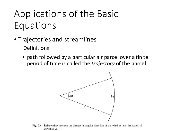
Applications of the Basic Equations • Trajectories and streamlines Definitions • path followed by a particular air parcel over a finite period of time is called the trajectory of the parcel

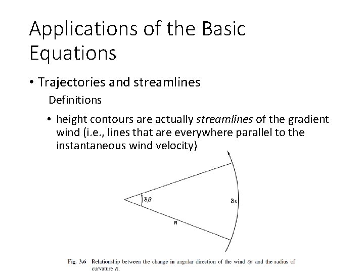
Applications of the Basic Equations • Trajectories and streamlines Definitions • height contours are actually streamlines of the gradient wind (i. e. , lines that are everywhere parallel to the instantaneous wind velocity)

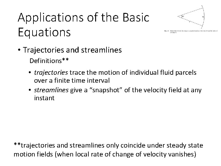
Applications of the Basic Equations • Trajectories and streamlines Definitions** • trajectories trace the motion of individual fluid parcels over a finite time interval • streamlines give a “snapshot” of the velocity field at any instant **trajectories and streamlines only coincide under steady state motion fields (when local rate of change of velocity vanishes)

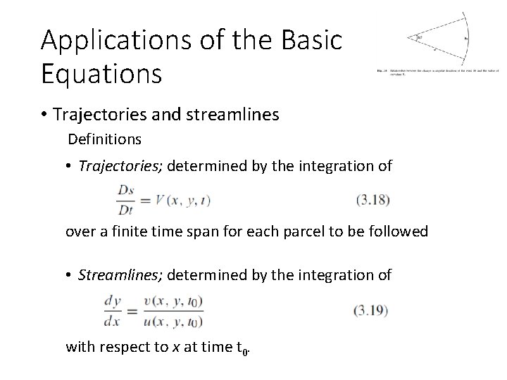
Applications of the Basic Equations • Trajectories and streamlines Definitions • Trajectories; determined by the integration of over a finite time span for each parcel to be followed • Streamlines; determined by the integration of with respect to x at time t 0 0

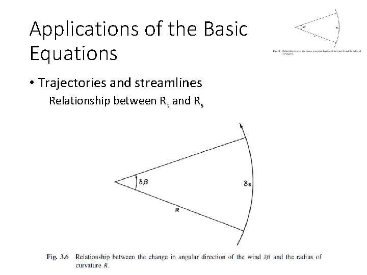
Applications of the Basic Equations • Trajectories and streamlines Relationship between Rt and Rs

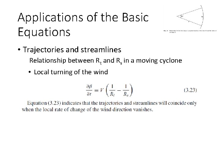
Applications of the Basic Equations • Trajectories and streamlines Relationship between Rt and Rs in a moving cyclone • Local turning of the wind

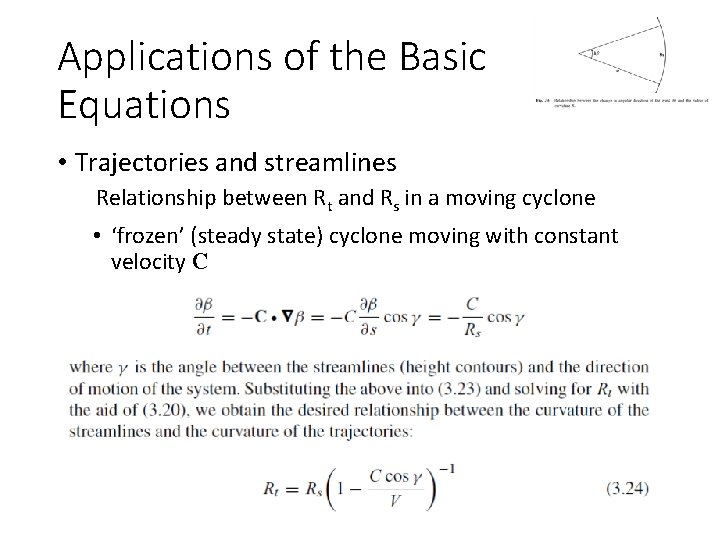
Applications of the Basic Equations • Trajectories and streamlines Relationship between Rt and Rs in a moving cyclone • ‘frozen’ (steady state) cyclone moving with constant velocity C

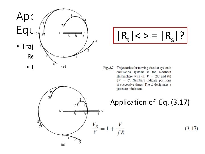
Applications of the Basic Equations |R |< > = |R |? • Trajectories and streamlines t s Relationship between Rt and Rs in a moving cyclone • Local turning of the wind Application of Eq. (3. 17)

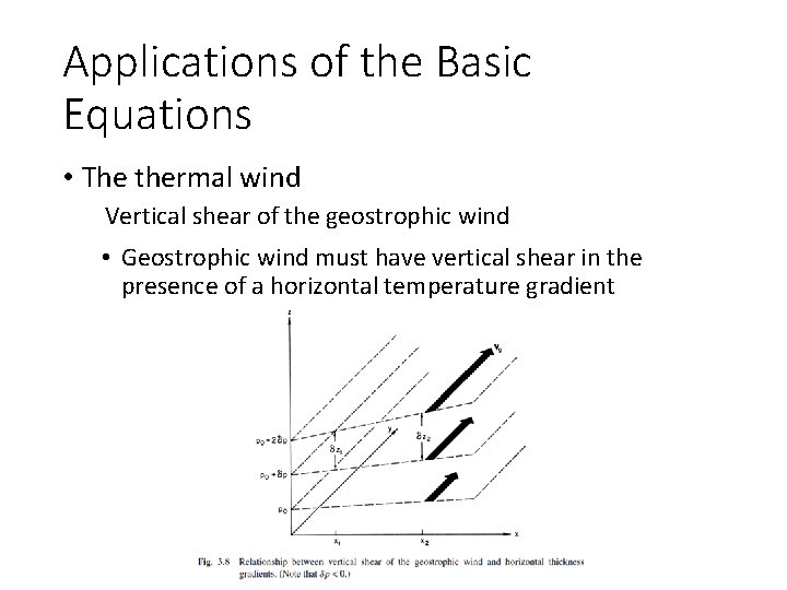
Applications of the Basic Equations • The thermal wind Vertical shear of the geostrophic wind • Geostrophic wind must have vertical shear in the presence of a horizontal temperature gradient

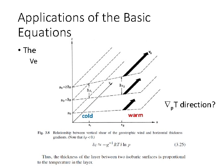
Applications of the Basic Equations • The thermal wind Vertical shear of the geostrophic wind p. T direction? cold warm

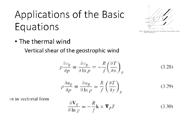
Applications of the Basic Equations • The thermal wind Vertical shear of the geostrophic wind

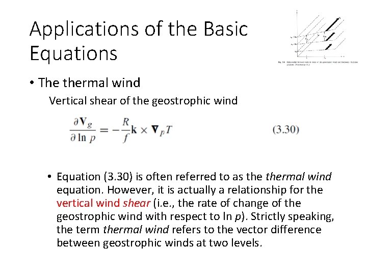
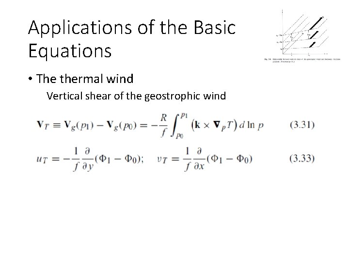
Applications of the Basic Equations • The thermal wind Vertical shear of the geostrophic wind • Equation (3. 30) is often referred to as thermal wind equation. However, it is actually a relationship for the vertical wind shear (i. e. , the rate of change of the geostrophic wind with respect to ln p). Strictly speaking, the term thermal wind refers to the vector difference between geostrophic winds at two levels.

Applications of the Basic Equations • The thermal wind Vertical shear of the geostrophic wind

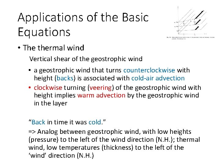
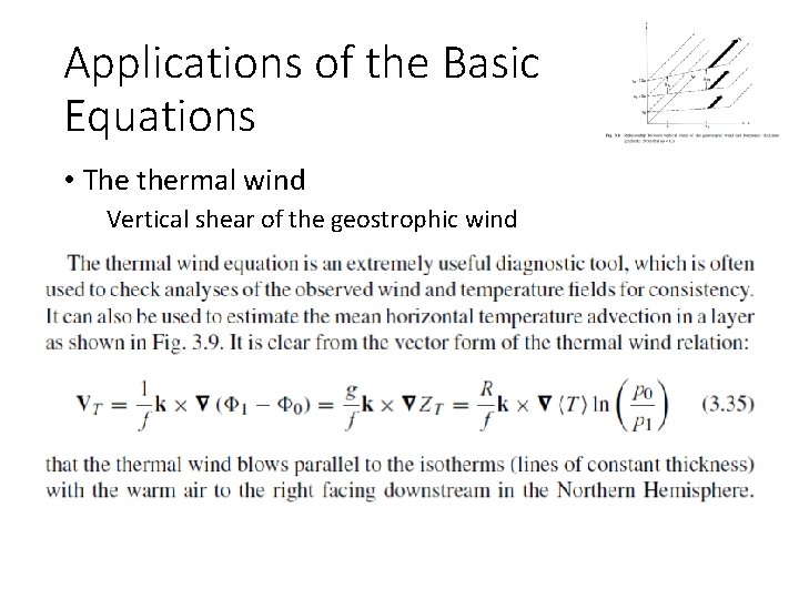
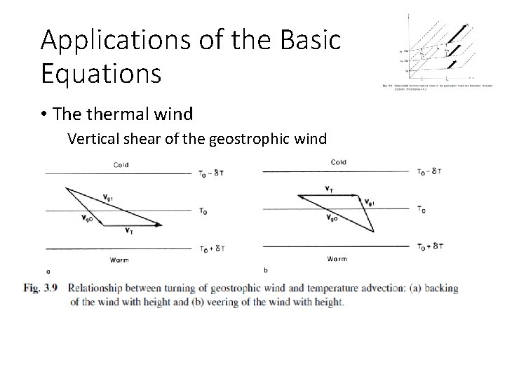
Applications of the Basic Equations • The thermal wind Vertical shear of the geostrophic wind • a geostrophic wind that turns counterclockwise with height (backs) is associated with cold-air advection • clockwise turning (veering) of the geostrophic wind with height implies warm advection by the geostrophic wind in the layer “Back in time it was cold. ” => Analog between geostrophic wind, with low heights (pressure) to the left of the wind direction (N. H. ); thermal wind, low temperatures (thickness) to the left of the ‘wind’ direction (N. H. )

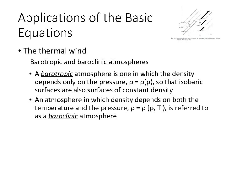
Applications of the Basic Equations • The thermal wind Barotropic and baroclinic atmospheres • A barotropic atmosphere is one in which the density depends only on the pressure, ρ = ρ(p), so that isobaric surfaces are also surfaces of constant density • An atmosphere in which density depends on both the temperature and the pressure, ρ = ρ (p, T ), is referred to as a baroclinic atmosphere

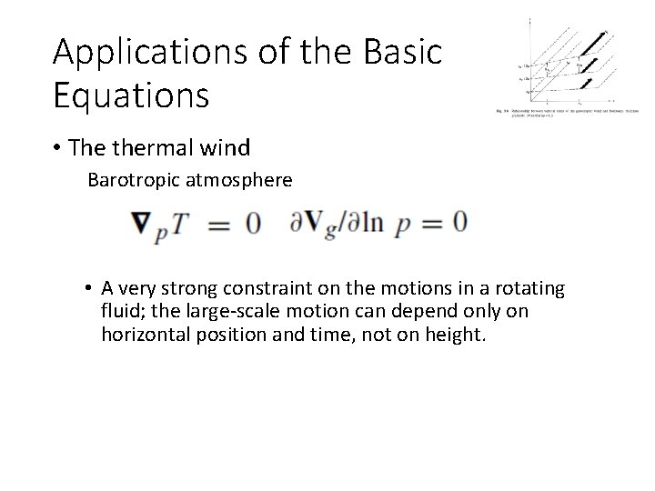
Applications of the Basic Equations • The thermal wind Barotropic atmosphere • A very strong constraint on the motions in a rotating fluid; the large-scale motion can depend only on horizontal position and time, not on height.

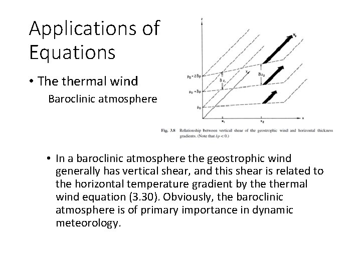
Applications of the Basic Equations • The thermal wind Baroclinic atmosphere • In a baroclinic atmosphere the geostrophic wind generally has vertical shear, and this shear is related to the horizontal temperature gradient by thermal wind equation (3. 30). Obviously, the baroclinic atmosphere is of primary importance in dynamic meteorology.

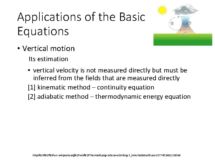
Applications of the Basic Equations • Vertical motion Its estimation • vertical velocity is not measured directly but must be inferred from the fields that are measured directly [1] kinematic method – continuity equation [2] adiabatic method – thermodynamic energy equation https%3 A%2 F%2 Fen. wikipedia. org%2 Fwiki%2 FThermal&psig=AOv. Vaw 2 JHIbng-3_kmx. Xbe 0 t 4 Lof&ust=1577652401134540

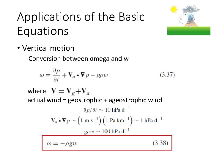
Applications of the Basic Equations • Vertical motion Conversion between omega and w where actual wind = geostrophic + ageostrophic wind

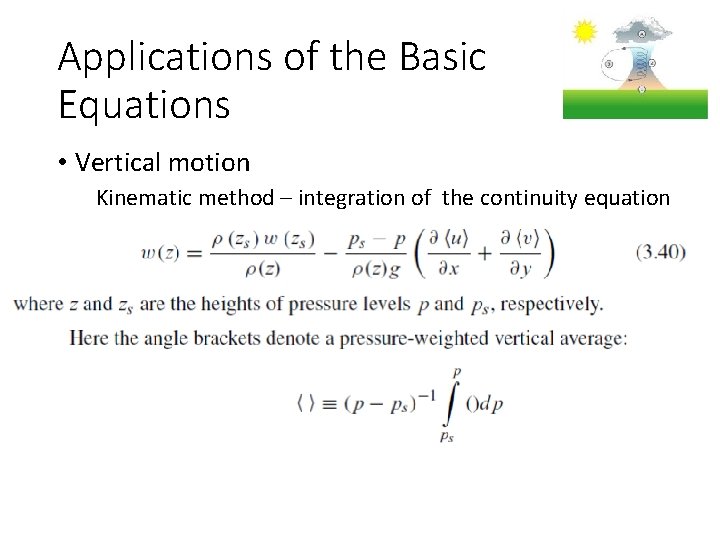
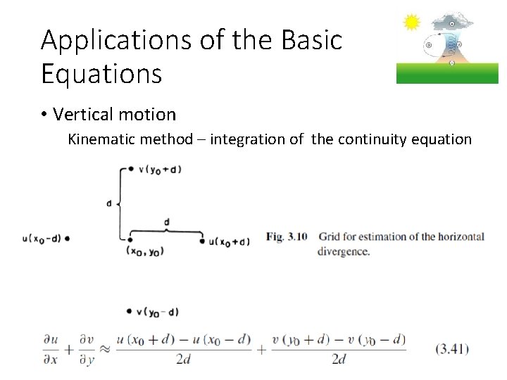
Applications of the Basic Equations • Vertical motion Kinematic method – integration of the continuity equation

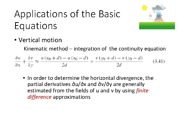
Applications of the Basic Equations • Vertical motion Kinematic method – integration of the continuity equation • In order to determine the horizontal divergence, the partial derivatives ∂u/∂x and ∂v/∂y are generally estimated from the fields of u and v by using finite difference approximations

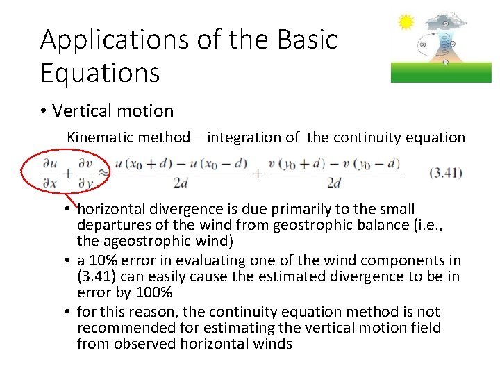
Applications of the Basic Equations • Vertical motion Kinematic method – integration of the continuity equation • horizontal divergence is due primarily to the small departures of the wind from geostrophic balance (i. e. , the ageostrophic wind) • a 10% error in evaluating one of the wind components in (3. 41) can easily cause the estimated divergence to be in error by 100% • for this reason, the continuity equation method is not recommended for estimating the vertical motion field from observed horizontal winds

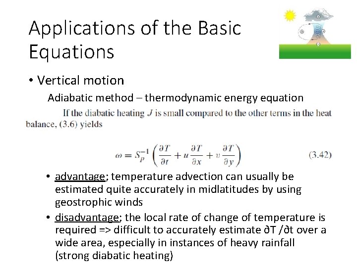
Applications of the Basic Equations • Vertical motion Adiabatic method – thermodynamic energy equation • advantage; temperature advection can usually be estimated quite accurately in midlatitudes by using geostrophic winds • disadvantage; the local rate of change of temperature is required => difficult to accurately estimate ∂T /∂t over a wide area, especially in instances of heavy rainfall (strong diabatic heating)

Applications of the Basic Equations • Computer weather model considerations Introduction [Chapter 13] • objective of a computer weather forecast model is to predict the future state of the atmospheric circulation from knowledge of its present state by use of numerical approximations to the dynamical equations https%3 A%2 F%2 Fwww. top 500. org%2 Fnews%2 Fjuwels-becomes-germanys-most-powerful-supercomputer%2 F&psig=AOv. Vaw 0 dz. V_m. Azim. ZYd. Ysx. JS 5 Nqe&ust=1577656927490960

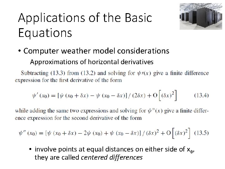
Applications of the Basic Equations • Computer weather model considerations Approximations of horizontal derivatives • involve points at equal distances on either side of x 0, they are called centered differences

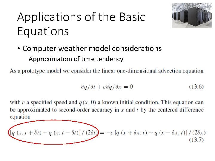
Applications of the Basic Equations • Computer weather model considerations Approximation of time tendency

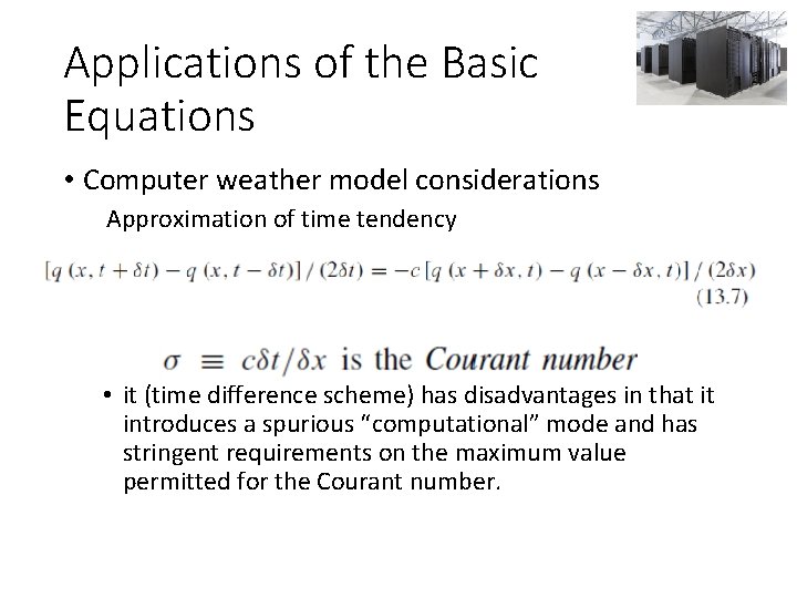
Applications of the Basic Equations • Computer weather model considerations Approximation of time tendency • it (time difference scheme) has disadvantages in that it introduces a spurious “computational” mode and has stringent requirements on the maximum value permitted for the Courant number.

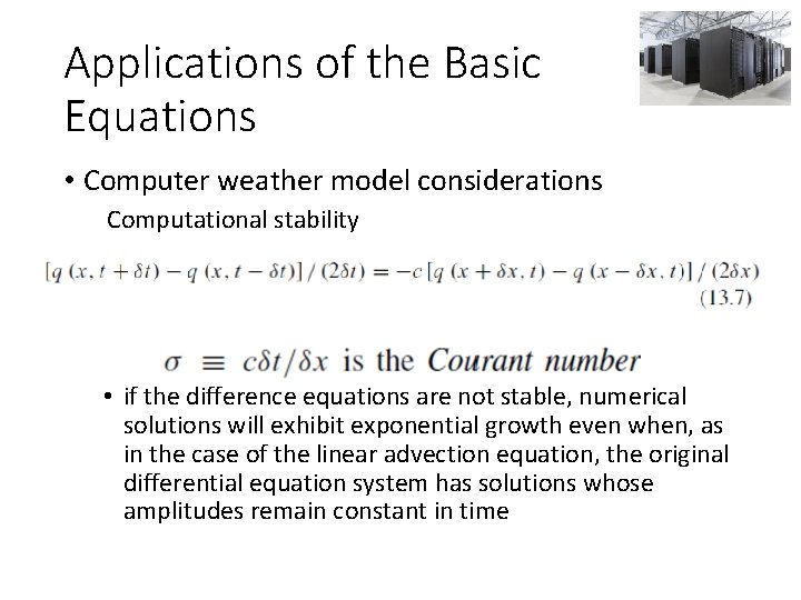
Applications of the Basic Equations • Computer weather model considerations Computational stability • if the difference equations are not stable, numerical solutions will exhibit exponential growth even when, as in the case of the linear advection equation, the original differential equation system has solutions whose amplitudes remain constant in time

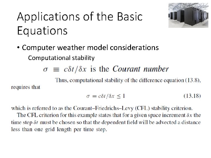
Applications of the Basic Equations • Computer weather model considerations Computational stability

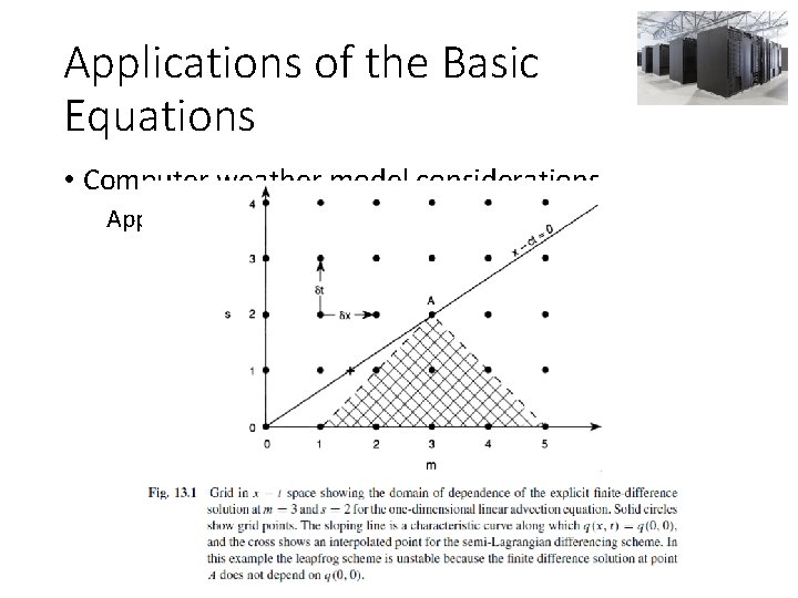
Applications of the Basic Equations • Computer weather model considerations Approximation of time tendency

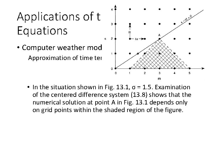
Applications of the Basic Equations • Computer weather model considerations Approximation of time tendency • In the situation shown in Fig. 13. 1, σ = 1. 5. Examination of the centered difference system (13. 8) shows that the numerical solution at point A in Fig. 13. 1 depends only on grid points within the shaded region of the figure.

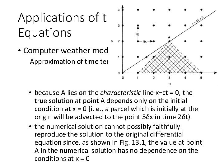
Applications of the Basic Equations • Computer weather model considerations Approximation of time tendency • because A lies on the characteristic line x−ct = 0, the true solution at point A depends only on the initial condition at x = 0 (i. e. , a parcel which is initially at the origin will be advected to the point 3δx in time 2δt) • the numerical solution cannot possibly faithfully reproduce the solution to the original differential equation since, as shown in Fig. 13. 1, the value at point A in the numerical solution has no dependence on the conditions at x = 0

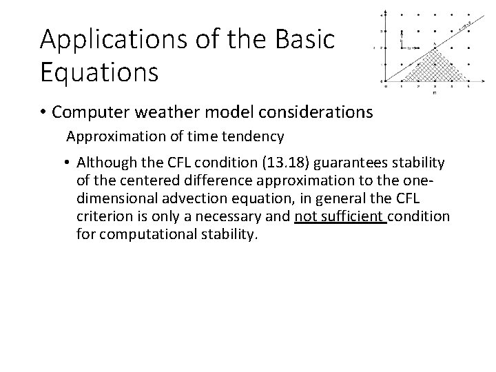
Applications of the Basic Equations • Computer weather model considerations Approximation of time tendency • Although the CFL condition (13. 18) guarantees stability of the centered difference approximation to the onedimensional advection equation, in general the CFL criterion is only a necessary and not sufficient condition for computational stability.

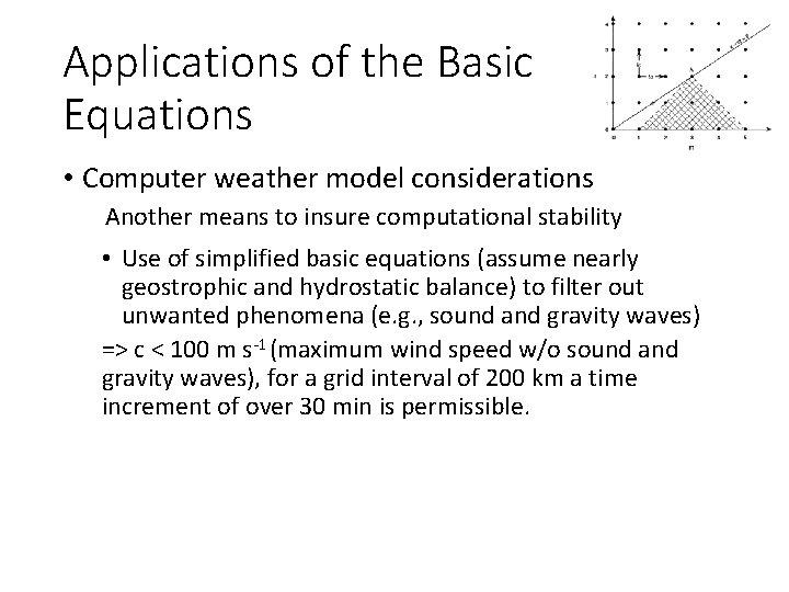
Applications of the Basic Equations • Computer weather model considerations Another means to insure computational stability • Use of simplified basic equations (assume nearly geostrophic and hydrostatic balance) to filter out unwanted phenomena (e. g. , sound and gravity waves) => c < 100 m s-1 (maximum wind speed w/o sound and gravity waves), for a grid interval of 200 km a time increment of over 30 min is permissible. − 1

Applications of the Basic Equations • Computer weather model considerations Lateral boundary conditions • Required for limited area models (e. g. , NAM, HRRR) • An outer ‘zone’ of blended fields from the forecast model and its ‘mother’ gridded fields (e. g. , GFS) • Allows the computation of horizontal derivatives along the outer edge of the model

Applications of the Basic Equations • Computer weather model considerations Initial conditions • Required for ALL computer weather models • Needed to start the time tendency portion of the governing equations • Data assimilation – process of creating initial conditions that are a blend of [1] observations at locations of observing platforms (e. g. , ASOS, satellites, radars) [2] a gridded ‘first guess’ field, typically an old forecast from a previous computer weather model simulation, at locations lacking observations

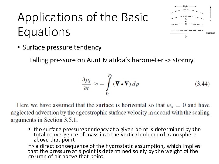
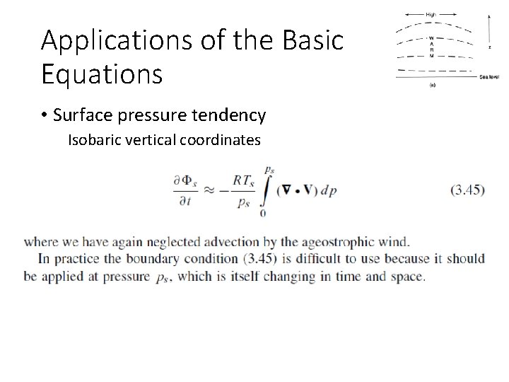
Applications of the Basic Equations • Surface pressure tendency Falling pressure on Aunt Matilda’s barometer -> stormy • the surface pressure tendency at a given point is determined by the total convergence of mass into the vertical column of atmosphere above that point => a direct consequence of the hydrostatic assumption, which implies that the pressure at a point is determined solely by the weight of the column of air above that point

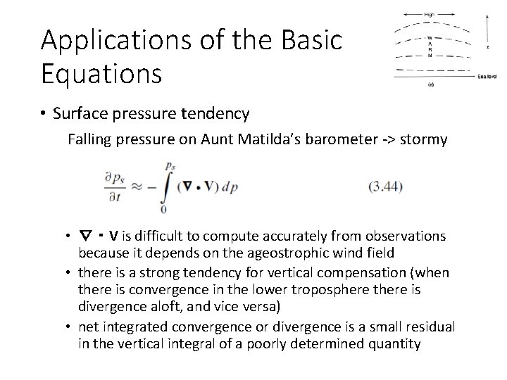
Applications of the Basic Equations • Surface pressure tendency Falling pressure on Aunt Matilda’s barometer -> stormy • ∇・V is difficult to compute accurately from observations because it depends on the ageostrophic wind field • there is a strong tendency for vertical compensation (when there is convergence in the lower troposphere there is divergence aloft, and vice versa) • net integrated convergence or divergence is a small residual in the vertical integral of a poorly determined quantity

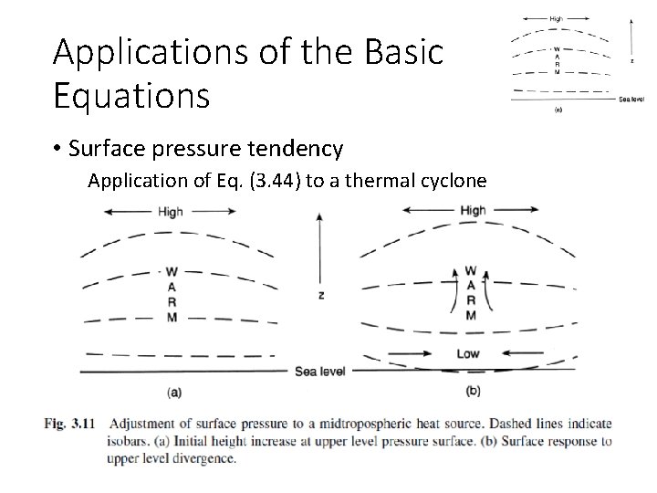
Applications of the Basic Equations • Surface pressure tendency Application of Eq. (3. 44) to a thermal cyclone

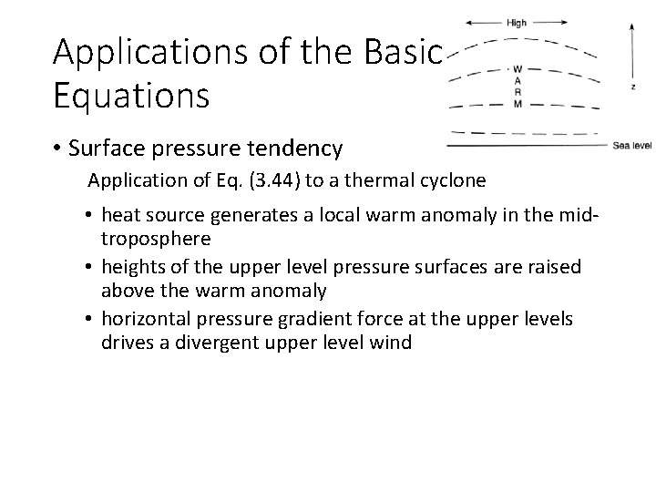
Applications of the Basic Equations • Surface pressure tendency Application of Eq. (3. 44) to a thermal cyclone • heat source generates a local warm anomaly in the midtroposphere • heights of the upper level pressure surfaces are raised above the warm anomaly • horizontal pressure gradient force at the upper levels drives a divergent upper level wind

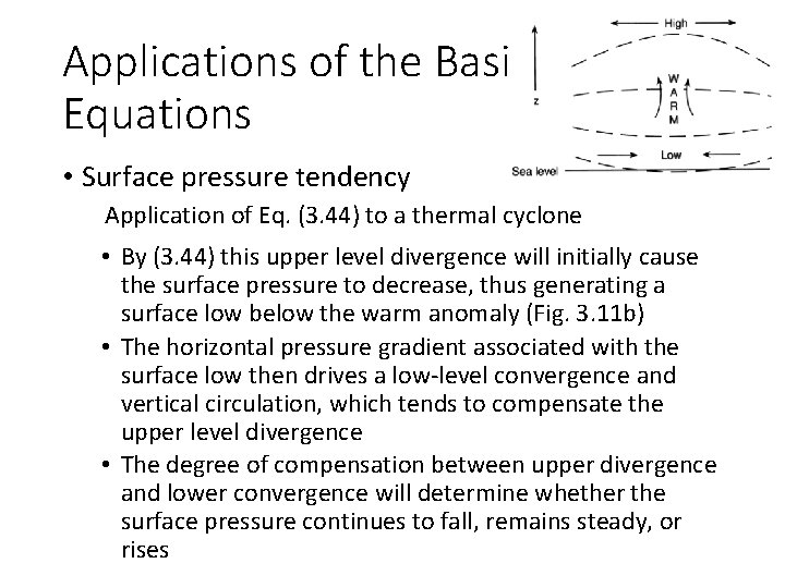
Applications of the Basic Equations • Surface pressure tendency Application of Eq. (3. 44) to a thermal cyclone • By (3. 44) this upper level divergence will initially cause the surface pressure to decrease, thus generating a surface low below the warm anomaly (Fig. 3. 11 b) • The horizontal pressure gradient associated with the surface low then drives a low-level convergence and vertical circulation, which tends to compensate the upper level divergence • The degree of compensation between upper divergence and lower convergence will determine whether the surface pressure continues to fall, remains steady, or rises

Applications of the Basic Equations • Surface pressure tendency Isobaric vertical coordinates