Applications of Modern Data Collection and Modelling Techniques

Applications of Modern Data Collection and Modelling Techniques to Biogeochemistry GGR 403 S Eugene Kwan March 2004

The Scientific Method

Data Acquisition • Remote Sensing • Isotopic Proxy Data/Mass Spectrometry • Eddy Correlation Techniques

Remote Sensing • Satellites, Airplanes, Ground-Based • Uses spectrometers: instruments which analyze different parts of the electromagnetic spectrum • “Passive vs. Active” Sensing – passive: satellite just gathers light – active: satellites emit energy

Satellite Orbits • Geostationary: satellite stays over the same part of the Earth at all times • Near-Polar: N/S orbits which, with the Earth’s E/W rotation, allow broad coverage • Sun-Synchronous: Each area of the world is covered at the same local sun time

Some Terminology • “swath”: the area on the surface a satellite can image at one time • “spatial resolution”: the size of the smallest feature that can be detected • “spectral resolution”: how far apart two spectral features must be in wavelength to be distinguished • “radiometric resolution”: how far apart two signals have to be in amplitude to be resolved

Types of Sensing • Optical/Stereoimages • Multi-Spectral • Thermal • Weather • Land-Observation

Stable Isotope Ratio Mass Spectrometry • “proxy data”: a series of measurements which from which various historical parameters may be inferred e. g. temperature may be inferred from oxygen isotope ratios in carbonates • typically used to reconstruct past climates

A Quick Review • Atoms contain protons (positive charge), neutrons (no charge), and electrons (negative charge) • The chemical properties of an atom depend principally on its atomic number: the number of protons • Atoms are neutral: # protons = # electrons

Isotopes • Isotope: - same number of protons and electrons - different number of neutrons - e. g. 16 O and 18 O are isotopes • absolutely not to be confused with allotrope, isomer, etc. • Stable vs. Unstable: unstable isotopes decay into stable ones over time (e. g. 13 C decays and is unstable while 12 C does not decay and is stable)

Isotopic Composition • elements naturally exist in a distribution of isotopic forms: natural abundance • non-equilibrium biological or physical processes can alter this distribution: fractionation e. g. Plant Photosynthesis plants prefer 12 C over 13 C by… C 3 plants 16 -18% C 4 plants 4%

Carbon Isotopic Composition • ref. : Coplen. Nature. 1995, 375, 285. • Reference is with respect to a special carbonate rock (NBS-19)

Measuring Isotopes with Mass Spectrometry 1) Sample is vaporized. 2) The gas is ionized, sometimes by bombarding it with electrons. 3) A magnetic field is used to separate the ions by mass: charge (m/z) ratio. 4) A detector measures the relative abundance of each m/z: gives a mass spectrum - technique is extremely sensitive

Missing Carbon Sink • carbon isotope fractionation can be used to distinguish between carbon dioxide fluxes between the land oceans • ocean-atmosphere CO 2 exchange: – insignificant fractionation • on-land CO 2 partitioning: – should result in noticeable d 13 C

Eddy Correlations • used to measure pollutant fluxes in the atmosphere • satellite measurements: – tend to measure total vertical concentrations (“atmospheric column”) – insufficient spatiotemporal resolution to calculate flux • “flux”: how much of something passes through a unit area per unit time

Fluid Flows • two regimes: laminar and turbulent • flows are empirically characterized by their Reynold’s Number Re:

Turbulent Flux • Mathematically, • CX and w fluctuate, so F fluctuates

Eddy Correlation Method

Data Analysis • “time series”: a set of measurements collected over time Techniques: - Smoothing - Detrending - Correlation/Autocorrelation/Convolution - Fourier Transform (FT)

Data Smoothing • • data typically too noisy to work with would like to smooth it so trends can be observed Two Methods: 1) Running Average/Running Mean 2) Running Median

Running Mean • visualization of a three-point running mean:

Running Median • Problem: what if there are anomalous spikes in the data? • outliers can totally swamp the average • Solution: use a running median reminder: median means “what’s the middle number”? (even number of points? average the middle two)

Example of Running Smoothing -magnetic observatory data courtesy Prof. Milkereit -graphs generated in Mathematica (by me) -although mean appears as good as median, a spectral analysis (see later) will show lower S/N

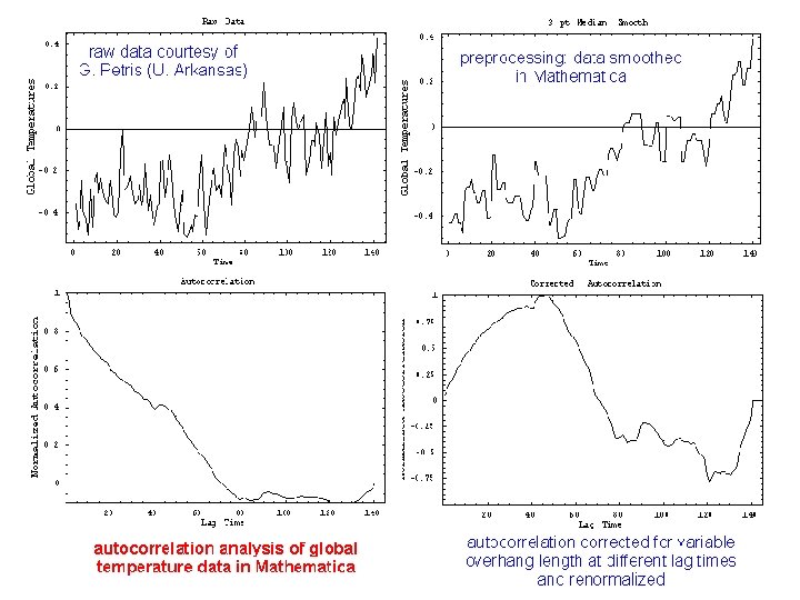
Correlation Methods • purposes: 1) find periodicities in data 2) relate two data sets 3) subtract instrumental effects Methods: - auto- and cross- correlation - convolution

Autocorrelation • Consider a discrete time series: f[t] = { f[t 0], f[t 0+D], f[t 0+2 D], … } where D is the sampling interval. Autocorrelation tries to determine how f[t] is related to f[t-D], f[t-2 D], … If f[t] depends on f[t-n. D], n=integer, then f[t] is “autocorrelated” with “lag time” n. D.

Meaning of Autocorrelation • Note that a “strong autocorrelation with lag time 2 Dt” means: – choose a f[t 1] – f[t 1 -2 Dt] is strongly related (same sign, magnitude) to f[t 1] – does not refer to particular times in the series

Cross-Correlation • Tries to find relationship between two different time series. • e. g. , sunspot activity and oceanic primary productivity. • Implementation: rather than copying the original series and calculating the shift overlaps, calculate the shift overlaps between the two time series.

Convolution/Deconvolution • Mathematically more complex • Useful for – Combining measurements taken from different instruments – Distinguishing real signals from instrumental noise • Its opposite, decovolution, can decompose two overlapping signals into their components.

Data Modelling • • • One Box Model Lifetime First-Order Approximation Steady States/Dynamic Equilibria Multibox Models/General Circulation Models

Data Extrapolation • Will consider the carbon cycle in terms of a simple multi-box model • Will account for p. H and solubility of carbon dioxide in the oceans • Will make some lifetime estimates and other predictions