APPLICATION OF NONLINEAR TIME SERIES ANALYSIS TECHNIQUES TO

APPLICATION OF NON-LINEAR TIME SERIES ANALYSIS TECHNIQUES TO THE NORDIC SPOT ELECTRICITY MARKET DATA Fernanda Strozzi, Eugénio Gutiérrez Tenrreiro and José-Manuel Zaldívar Comenges Update on WP 5: Task 5. 2 Deliverable 5. 3

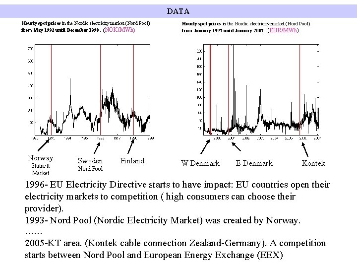
DATA Hourly spot prices in the Nordic electricity market (Nord Pool) from May 1992 until December 1998. (NOK/MWh) Norway Statnett Market Sweden Nord Pool Finland Hourly spot prices in the Nordic electricity market (Nord Pool) from January 1997 until January 2007. (EUR/MWh) W Denmark E Denmark Kontek 1996 - EU Electricity Directive starts to have impact: EU countries open their electricity markets to competition ( high consumers can choose their provider). 1993 - Nord Pool (Nordic Electricity Market) was created by Norway. …… 2005 -KT area. (Kontek cable connection Zealand-Germany). A competition starts between Nord Pool and European Energy Exchange (EEX)

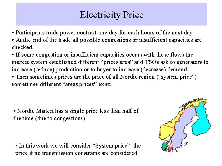
Electricity Price • Participants trade power contract one day for each hours of the next day • At the end of the trade all possible congestions or insufficient capacities are checked. • If some congestion or insufficient capacities occurs with these flows the market system established different “prices area” and TSOs ask to generators to increase (reduce) production or to buyer to increase (decrease) demand. • Then sometimes prices are the price of all Nordic region (“system price”) sometimes different “areas prices” exist. • Nordic Market has a single price less than half of the time (due to congestions) • In this work we will consider “System price”: the price if no transmission constrains are considered

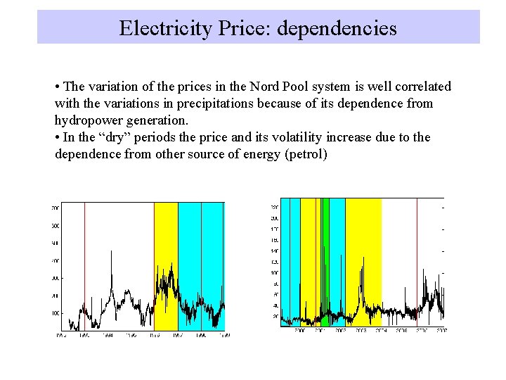
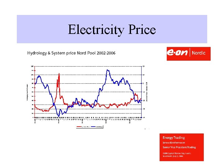
Electricity Price: dependencies • The variation of the prices in the Nord Pool system is well correlated with the variations in precipitations because of its dependence from hydropower generation. • In the “dry” periods the price and its volatility increase due to the dependence from other source of energy (petrol)

Electricity Price

Goals 1. Characterizing time series spot price dynamics comparing them with - Linear Gaussian dynamic with the same fft testing nonlinearity - Time series with the same probability distribution but not temporally correlated (shuffled) 2. Detect important events using nonlinear time series analysis

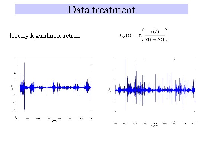
Data treatment Hourly logarithmic return

Hurst exponent: H H provides a measure of whether the data are a pure random walk or have some trend (i. e. some degree of correlation exists) H is a tool for studying long-term memory and fractality of a time series A long memory process is a process with a random component, where a past event has a slow decaying effect on future events.

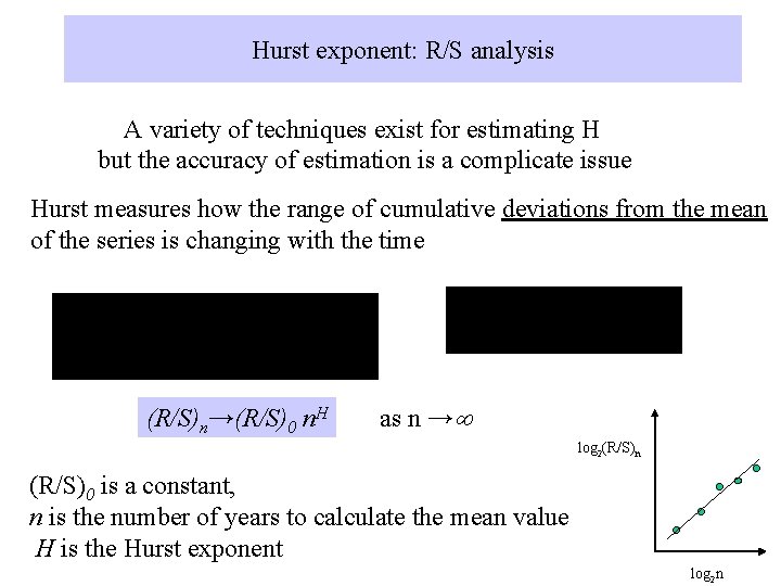
Hurst exponent: R/S analysis A variety of techniques exist for estimating H but the accuracy of estimation is a complicate issue Hurst measures how the range of cumulative deviations from the mean of the series is changing with the time . (R/S)n→(R/S)0 n. H as n → log 2(R/S)n (R/S)0 is a constant, n is the number of years to calculate the mean value H is the Hurst exponent log 2 n

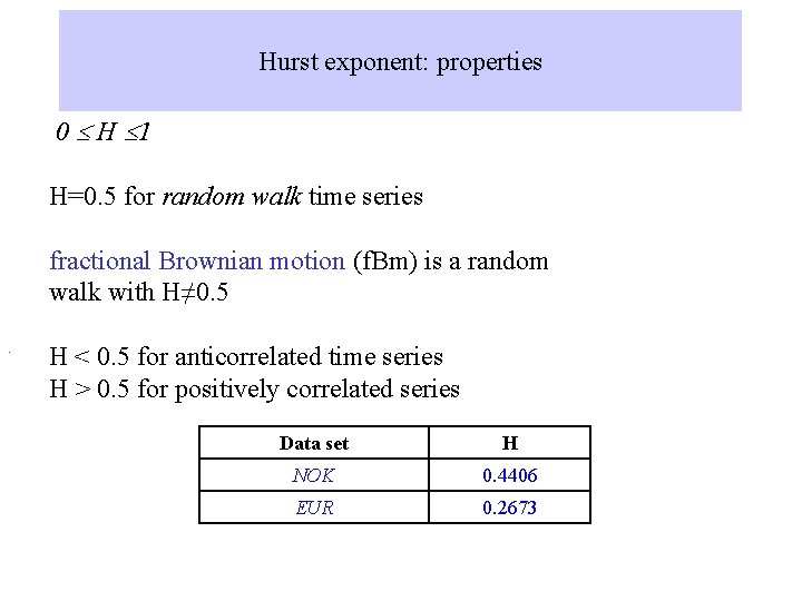
Hurst exponent: properties 0 H 1 H=0. 5 for random walk time series fractional Brownian motion (f. Bm) is a random walk with H≠ 0. 5. H < 0. 5 for anticorrelated time series H > 0. 5 for positively correlated series Data set H NOK 0. 4406 EUR 0. 2673

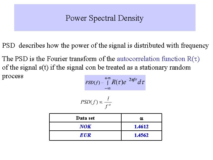
Power Spectral Density PSD describes how the power of the signal is distributed with frequency The PSD is the Fourier transform of the autocorrelation function R(t) of the signal s(t) if the signal con be treated as a stationary random process Data set a NOK 1. 4612 EUR 1. 4562

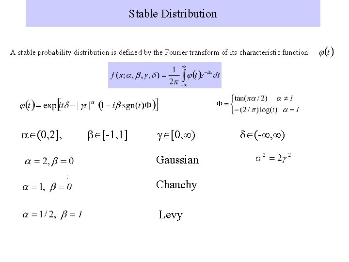
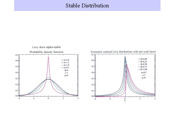
Stable Distribution A stable probability distribution is defined by the Fourier transform of its characteristic function a (0, 2], b [-1, 1] g [0, ) Gaussian : Chauchy Levy d (- , )

Stable Distribution

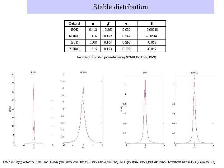
Stable distribution Data set a b g. d NOK 0. 412 -0. 365 0. 035 -0. 00018 NOK(0) 1. 116 0. 127 0. 242 -0. 0514 EUR 1. 308 0. 164 0. 268 -0. 068 EUR(0) 1. 315 0. 173 0. 272 -0. 069 Nord Pool data fitted parameters using STABLE (Nolan, 1999). Fitted density plot for the Nord Pool Norwegian Krone and Euro time series data (blue line): a/Original time series, first difference; b/ without zero values (23962 values).

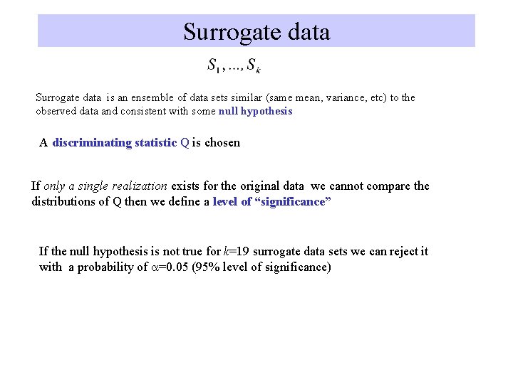
Surrogate data is an ensemble of data sets similar (same mean, variance, etc) to the observed data and consistent with some null hypothesis A discriminating statistic Q is chosen If only a single realization exists for the original data we cannot compare the distributions of Q then we define a level of “significance” If the null hypothesis is not true for k=19 surrogate data sets we can reject it with a probability of a=0. 05 (95% level of significance)

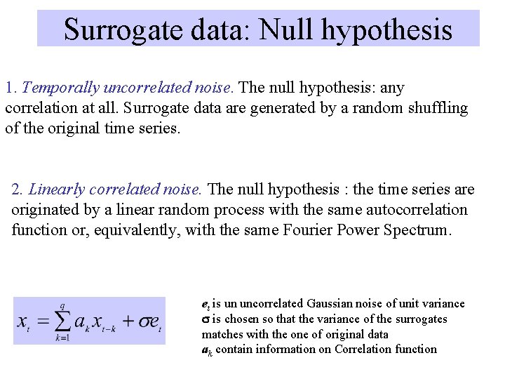
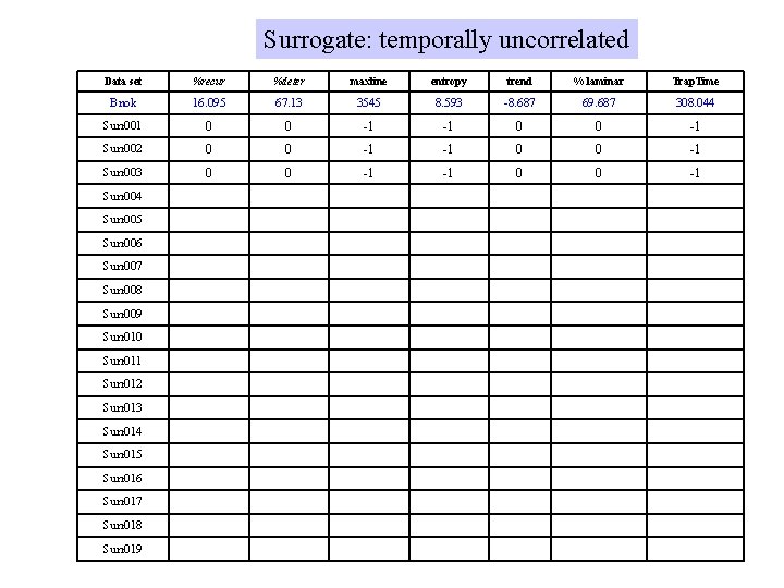
Surrogate data: Null hypothesis 1. Temporally uncorrelated noise. The null hypothesis: any correlation at all. Surrogate data are generated by a random shuffling of the original time series. 2. Linearly correlated noise. The null hypothesis : the time series are originated by a linear random process with the same autocorrelation function or, equivalently, with the same Fourier Power Spectrum. et is un uncorrelated Gaussian noise of unit variance s is chosen so that the variance of the surrogates matches with the one of original data ak contain information on Correlation function

Surrogate data: discriminating statistic Q The dynamic is chaotic? Q = Correlation dimension Q = Lyapunov exponent Q = Forecasting error The structures of recurrence plots? Q = RQA measures

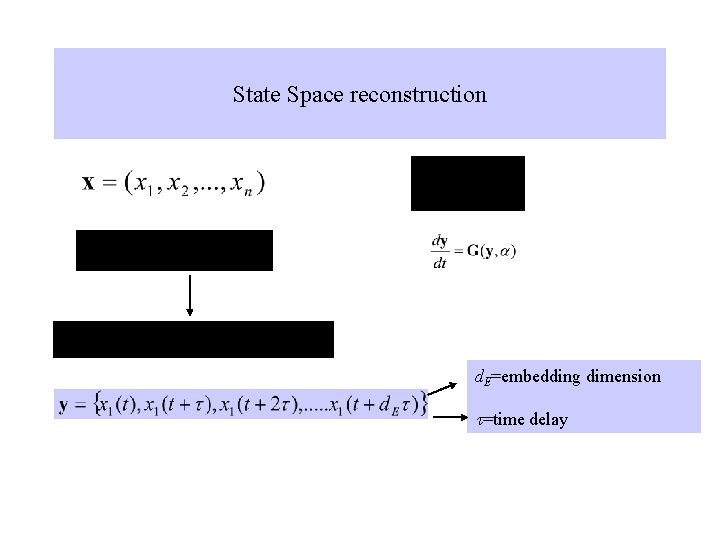
State Space reconstruction d. E=embedding dimension t=time delay

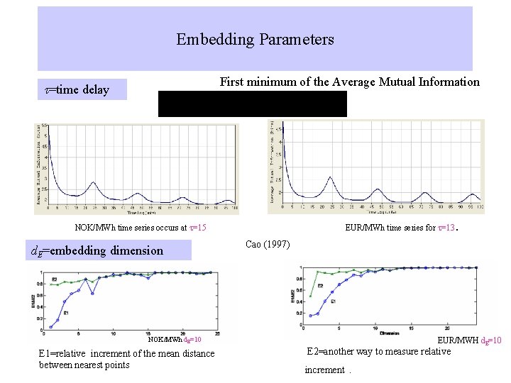
Embedding Parameters First minimum of the Average Mutual Information t=time delay . NOK/MWh time series occurs at t=15 d. E=embedding dimension EUR/MWh time series for t=13 Cao (1997) NOK/MWh d. E=10 E 1=relative increment of the mean distance between nearest points EUR/MWH d. E=10 E 2=another way to measure relative increment.

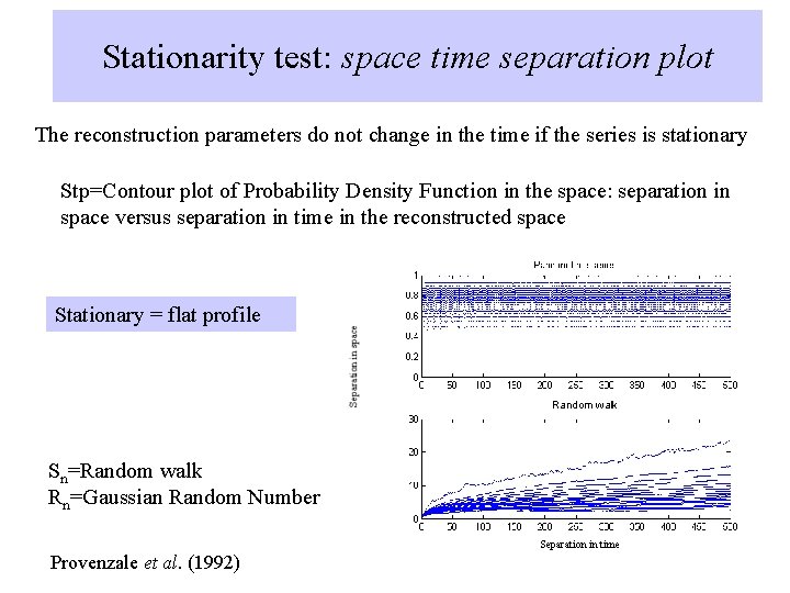
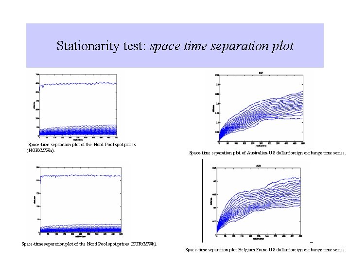
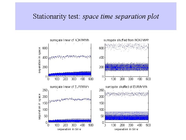
Stationarity test: space time separation plot The reconstruction parameters do not change in the time if the series is stationary Stp=Contour plot of Probability Density Function in the space: separation in space versus separation in time in the reconstructed space Stationary = flat profile Random walk Sn=Random walk Rn=Gaussian Random Number Separation in time Provenzale et al. (1992)

Stationarity test: space time separation plot Space-time separation plot of the Nord Pool spot prices (NOK/MWh). Space-time separation plot of Australian-US dollar foreign exchange time series. Space-time separation plot of the Nord Pool spot prices (EUR/MWh). Space-time separation plot Belgium Franc-US dollar foreign exchange time series.

Stationarity test: space time separation plot

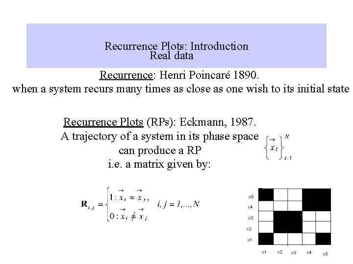
Recurrence Plots: Introduction Real data Recurrence: Henri Poincaré 1890. when a system recurs many times as close as one wish to its initial state Recurrence Plots (RPs): Eckmann, 1987. A trajectory of a system in its phase space can produce a RP i. e. a matrix given by:

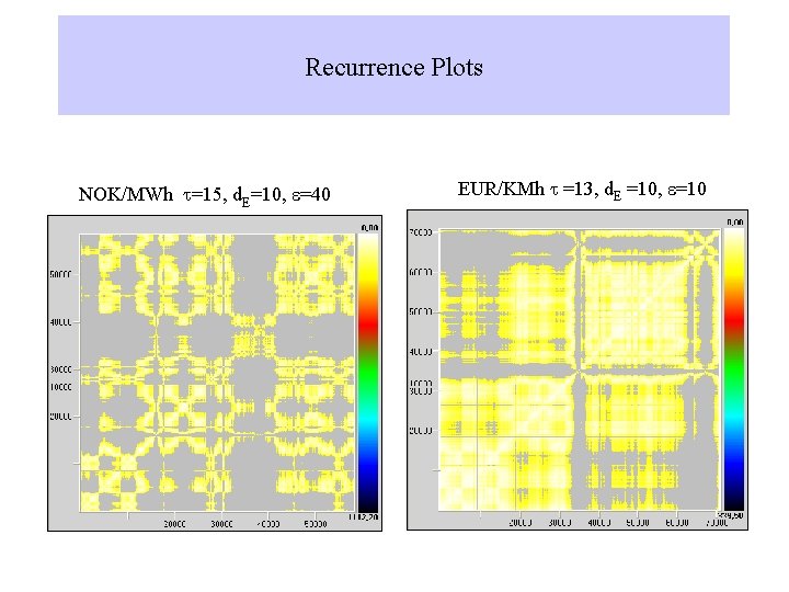
Recurrence Plots NOK/MWh t=15, d. E=10, e=40 EUR/KMh t =13, d. E =10, e=10

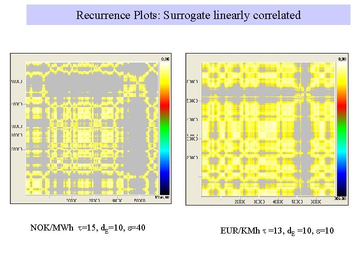
Recurrence Plots: Surrogate linearly correlated NOK/MWh t=15, d. E=10, e=40 EUR/KMh t =13, d. E =10, e=10

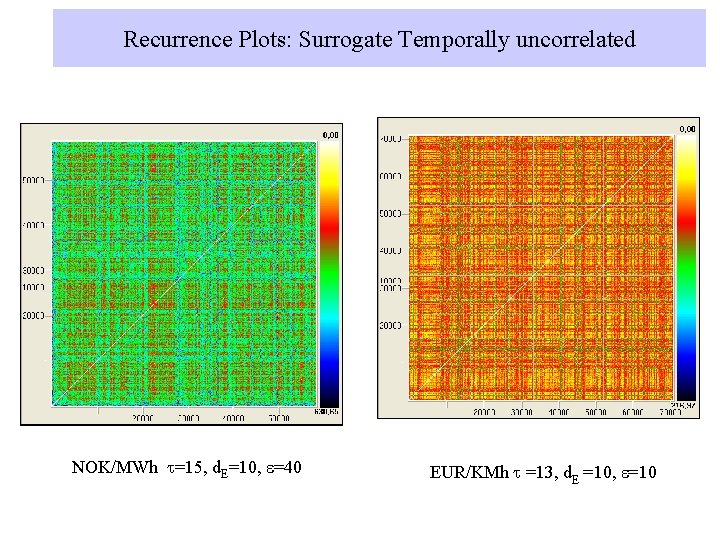
Recurrence Plots: Surrogate Temporally uncorrelated NOK/MWh t=15, d. E=10, e=40 EUR/KMh t =13, d. E =10, e=10

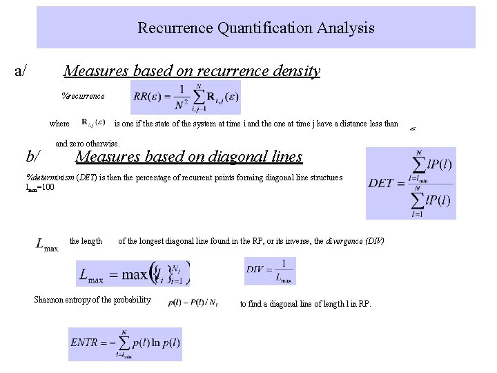
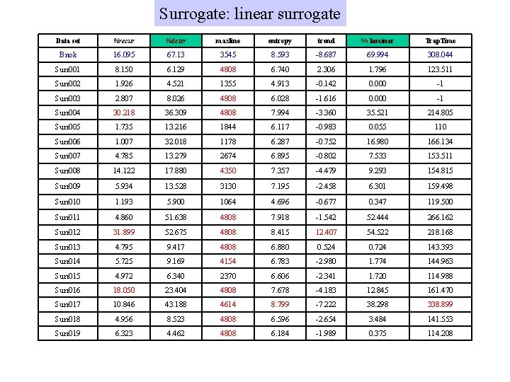
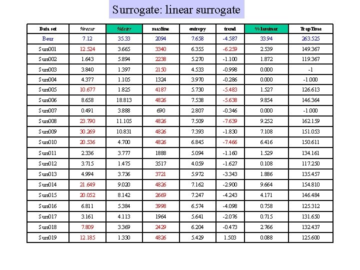
Recurrence Quantification Analysis a/ Measures based on recurrence density %recurrence where b/ is one if the state of the system at time i and the one at time j have a distance less than and zero otherwise. Measures based on diagonal lines %determinism (DET) is then the percentage of recurrent points forming diagonal line structures lmin=100 the length of the longest diagonal line found in the RP, or its inverse, the divergence (DIV) Shannon entropy of the probability to find a diagonal line of length l in RP.

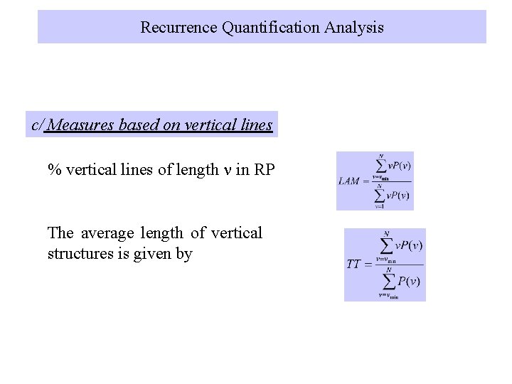
Recurrence Quantification Analysis c/ Measures based on vertical lines % vertical lines of length n in RP The average length of vertical structures is given by

Surrogate: linear surrogate Data set %recur %deter maxline entropy trend % laminar Trap. Time Bnok 16. 095 67. 13 3545 8. 593 -8. 687 69. 994 308. 044 Surr 001 8. 150 6. 129 4808 6. 740 2. 306 1. 796 123. 511 Surr 002 1. 926 4. 521 1355 4. 913 -0. 142 0. 000 -1 Surr 003 2. 807 8. 026 4808 6. 028 -1. 616 0. 000 -1 Surr 004 30. 218 36. 309 4808 7. 994 -3. 360 35. 521 214. 805 Surr 005 1. 735 13. 216 1844 6. 117 -0. 983 0. 055 110 Surr 006 1. 007 32. 018 1178 6. 287 -0. 752 16. 980 166. 134 Surr 007 4. 785 13. 279 2674 6. 895 -0. 802 7. 533 153. 511 Surr 008 14. 122 17. 880 4350 7. 357 -4. 479 9. 293 154. 815 Surr 009 5. 934 13. 528 3130 7. 195 -2. 458 6. 301 159. 498 Surr 010 1. 193 5. 900 1064 4. 696 -0. 677 0. 347 119. 500 Surr 011 4. 860 51. 638 4808 7. 918 -1. 542 52. 444 266. 162 Surr 012 31. 899 52. 675 4808 8. 415 12. 407 54. 522 218. 168 Surr 013 4. 795 9. 417 4808 6. 880 0. 524 0. 724 143. 393 Surr 014 5. 725 9. 169 4154 6. 783 -2. 980 1. 774 144. 963 Surr 015 4. 972 6. 340 2370 6. 606 -2. 341 1. 720 114. 988 Surr 016 18. 050 23. 404 4808 7. 678 -4. 183 12. 845 161. 470 Surr 017 10. 846 43. 188 4614 8. 799 -7. 222 38. 298 338. 899 Surr 018 4. 956 8. 523 4808 6. 596 -2. 654 3. 484 141. 553 Surr 019 6. 323 4. 462 4808 6. 184 -1. 989 0. 375 114. 208

Surrogate: linear surrogate Data set %recur %deter maxline entropy trend % laminar Trap. Time Beur 7. 12 35. 33 2094 7. 658 -4. 587 33. 94 263. 525 Surr 001 12. 524 3. 665 3340 6. 355 -6. 259 2. 539 149. 367 Surr 002 1. 643 5. 894 2238 5. 270 -1. 100 1. 872 119. 367 Surr 003 3. 840 1. 397 2150 4. 533 -0. 998 0. 000 -1 Surr 004 4. 377 1. 105 1324 3. 970 -0. 286 0. 000 -1. 000 Surr 005 10. 677 1. 825 4187 5. 730 -5. 483 1. 527 126. 613 Surr 006 8. 658 18. 813 4826 7. 538 -5. 638 9. 854 146. 364 Surr 007 0. 491 3. 888 690 2. 807 -0. 346 0. 000 -1. 000 Surr 008 23. 790 11. 105 4826 7. 509 -7. 639 9. 252 162. 159 Surr 009 30. 269 10. 831 4826 7. 393 -1. 830 7. 108 151. 053 Surr 010 20. 536 4. 700 4826 6. 845 -7. 466 6. 416 150. 611 Surr 011 2. 336 3. 777 1888 5. 094 -1. 160 1. 529 134. 161 Surr 012 3. 715 1. 475 3517 4. 059 -1. 627 0. 108 117. 250 Surr 013 4. 994 3. 736 3721 5. 972 -3. 343 1. 886 135. 457 Surr 014 21. 649 9. 020 4826 7. 162 -2. 900 9. 664 154. 810 Surr 015 20. 052 8. 142 2669 7. 247 -4. 243 4. 171 146. 484 Surr 016 6. 811 5. 384 3998 6. 574 -4. 098 0. 758 125. 312 Surr 017 3. 161 4. 113 1964 5. 641 -2. 076 0. 715 131. 650 Surr 018 7. 809 3. 369 2429 6. 204 -0. 473 2. 766 132. 437 Surr 019 12. 185 1. 330 4826 5. 429 1. 503 0. 088 125. 600

Surrogate: temporally uncorrelated Data set %recur %deter maxline entropy trend % laminar Trap. Time Bnok 16. 095 67. 13 3545 8. 593 -8. 687 69. 687 308. 044 Surr 001 0 0 -1 -1 0 0 -1 Surr 002 0 0 -1 -1 0 0 -1 Surr 003 0 0 -1 -1 0 0 -1 Surr 004 Surr 005 Surr 006 Surr 007 Surr 008 Surr 009 Surr 010 Surr 011 Surr 012 Surr 013 Surr 014 Surr 015 Surr 016 Surr 017 Surr 018 Surr 019

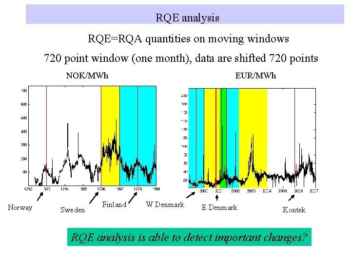
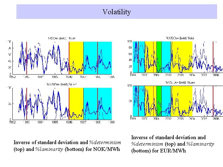
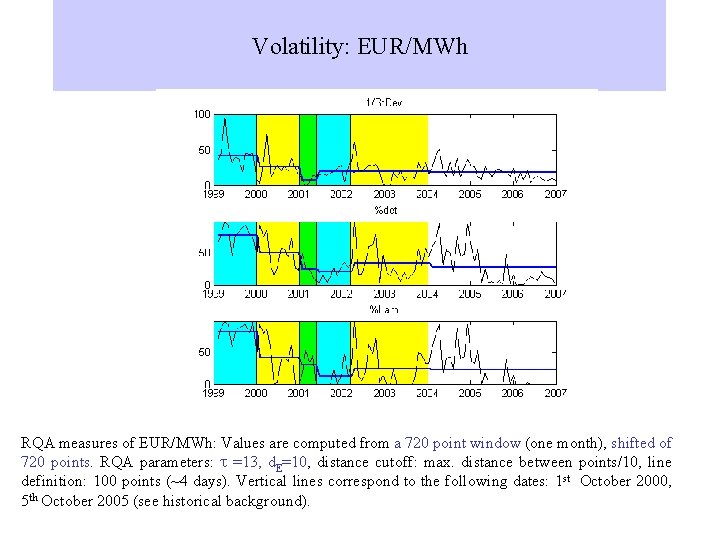
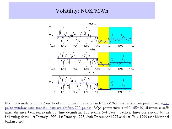
RQE analysis RQE=RQA quantities on moving windows 720 point window (one month), data are shifted 720 points NOK/MWh Norway Sweden Finland EUR/MWh W Denmark E Denmark Kontek RQE analysis is able to detect important changes?

Volatility Inverse of standard deviation and %determinism (top) and %laminarity (bottom) for NOK/MWh Inverse of standard deviation and %determinism (top) and %laminarity (bottom) for EUR/MWh

Volatility: EUR/MWh RQA measures of EUR/MWh: Values are computed from a 720 point window (one month), shifted of 720 points. RQA parameters: t =13, d. E=10, distance cutoff: max. distance between points/10, line definition: 100 points (~4 days). Vertical lines correspond to the following dates: 1 st October 2000, 5 th October 2005 (see historical background).

Volatility: NOK/MWh Nonlinear metrics of the Nord Pool spot prices time series in NOK/MWh: Values are computed from a 720 point window (one month), data are shifted 720 points. RQA parameters: t =15, d. E=10, distance cutoff: max. distance between points/10, line definition: 100 points (~4 days). Vertical lines correspond to the following dates: 1 st January 1993, 1 st January 1996, 29 th December 1997 and 1 st July 1999 (see historical background).

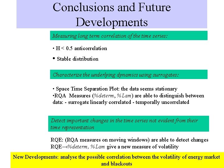
Conclusions and Future Developments Measuring long term correlation of the time series: • H < 0. 5 anticorrelation • Stable distribution Characterize the underlying dynamics using surrogates: • Space Time Separation Plot: the data seems stationary • RQA Measures (%determ, %Lam) are able to distinguish between data: - surrogate linearly correlated - temporally uncorrelated Detect important changes in the time series not evident from their time representation RQE: (RQA measures on moving windows) are able to detect changes RQE→%determ, %Lam give a new measure of volatility New Developments: analyse the possible correlation between the volatility of energy market and blackouts

Bibliography Data History: Amundsen, E. S. and Bergman, L. , 2007, Integration of multiple national markets for electricity: The case of Norway and Sweden, Energy Policy, doi. 1016/j. enpol. 2006. 12. 014. Byström H. N. E. 2005. Extreme value theory and extremely large electricity price changes. International Review of Economics and Finance 14, 41 -55. Hsieh, D. A. , Chaos and nonlinear dynamics: Application to financial markets, 1991, The Journal of Finance 46, 1839 -1887 Kristiansen, T. , 2007. Pricing of monthly contracts in the Nord Pool market. Energy Policy 35, 307 -316. Kristiansen, T. , 2006, A preliminary assessment of the market coupling arrangement on the Kontek cable, Energy Policy (in press) Perelló, J. , Montero, M. , Palatella, L. , Simonsen, I. and Masoliver, J. , 2007. Entropy of the Nordic electricity market: anomalous scaling, spikes, and mean-reversion. J. Stat. Physics (in press). Vehviläinen I. and Pyykkönen, T. 2005. Stochastic factor model for electricity spot price-the case of the Nordic market. Energy Economics 27, 351 -357. Weron, R. , Bierbrauer, M. and Truck, S. 2004. Modelling electricity prices: Jump diffusion and regime switching. Physica A 336, 39 -48.

Bibliography Hurst: Cannon, M. J. Percival, D. B. , Caccia, D. C. , Raymond, G. M. and Bassingthwaighte, J. B. , 1997, Evaluating scaled windowed variance methods for estimating the Hurst coefficient of time serie Haldrup, N. , Nielsen, M. Ø. , 2006. A regime switching long memory model for electricity prices. Journal of econometrics 135, 349 -376. Hurst, H. E. , 1951, Long-term storage capacity of reservoirs, Trans. Am. Soc. Civ. Eng. 116, 770 -779. Simonsen, I. , 2003. Measuring anti-correlations in the Nordic electricity spot market by wavelets. Physica A 322, 597 -606. Weron, R. and Przybyłowicz, B. , 2000. Hurst analysis of electricity price dynamics. Physica A 283, 462 -468. Embedding parameters Cao, L. , 1997, Practical method for determining the minimum embedding dimension of a scalar time series, Physica D 110, 43 -50. Surrogate data: Schreiber, T. and Schmitz, A. , 2000, Surrogate time series, Physica D 142, 346 -382. Theiler, J. , Eubank, S. , Longtin, A. , Galdrikian, B. , and Farmer, J. D. , 1992, Testing for nonlinearity in time series: the method of surrogate data. Physica D 58, 77 -. Space time separation plot: Hegger, R. , Kantz, H. , Schreiber, T. , 1999, Practical implementation of nonlinear time series methods: The TISEAN package. CHAOS 9, 413 -. The software package is publicly available at http: //www. mpipks-dresden. mpg. de/~tisean. Provenzale, A. , Smith, L. A. , Vio, R. and Murante, G. , 1992, Distinguishing between low-dimensional dynamics and randomness in measured time series. Physica D 58, 31 -49.

Bibliography Stable distributions: Nolan, J. P. , 1999. Fitting data and assessing goodness of fit with stable distributions. In Proceedings of the Conference on Applications of Heavy Tailed Distributions in Economics, Engineering and Statistics, American University, Washington DC, June 3 -5. Nolan, J. P. , 1997. Numerical computation of stable densities and distribution functions. Commun. Stat. : Stochastic models 13, 759 -774. PSD Theiler, J. , 1991, Some comments on the correlation dimension of noise. Phys. Lett A 155, 480 -493 . Recurrence plot: Eckmann, J. P. , Kamphorst, S. O. and Ruelle, D. , 1987, Recurrence plots of dynamical systems, Europhys. Lett. 4, 973977. Marwan, N. , Romano, M. C. , Thiel, M. and Kurths, J. , 2007. Recurrence plots for the analysis of complex systems. Physics Reports 438, 237 -329. Strozzi, F. , Zaldivar, J, M. , Zbilut, J. , P. , 2007, Recurrence quantification analysis and state space divergence reconstruction for financial time series analysis. Physica A 376, 487 -499 Strozzi, F. , Zaldívar, J. M. , & Zbilut, J. P. , 2002. Application of nonlinear time series analysis techniques to high frequency currency exchange data, Physica A 312, 520 -538. Zbilut, J. P. and Webber Jr. C. L. , 1992, Embeddings and delays as derived from quantification of recurrence plots. Phys. Lett. A 171, 199 -203