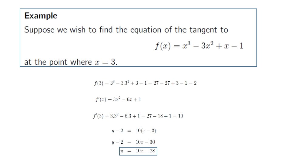
Application of Differentation Equation of the tangent line

Application of Differentation

Equation of the tangent line to the graph of the function

EXERCISES

Rolle’s Theorem Rolle's theorem is an important basic result about differentiable functions. Like many basic results in the calculus it seems very obvious. It just says that between any two points where the graph of the differentiable function f (x) cuts the horizontal line there must be a point where f '(x) = 0. The following picture illustrates theorem.

Rolle’s Theorem If 1) f (x) is continuous on [a, b], 2) f (x) is differentiable on (a, b), and 3) f (a) = f (b) then there is at least one value off isx continuous on (a, on [a, b] b), call it c, such that differentiable on (a, b) f(a) = f(b) f ’(c) = 0. a b

Example 1 ( f is continuous and differentiable) Since , then Rolle’s Theorem applies… then, x = – 1 , x = 0, and x = 1

Mean Value Theorem- MVT The Mean Value Theorem is one of the most important theoretical tools in Calculus. It states that if f(x) is defined and continuous on the interval [a, b] and differentiable on (a, b), then there is at least one number c in the interval (a, b) (that is a<c<b) such that In other words, there exists a point in the interval (a, b) which has a horizontal tangent. In fact, the Mean Value Theorem can be stated also in terms of slopes. Indeed, the number is the slope of the line passing through (a, f(a)) and (b, f(b)). So the conclusion of the Mean Value Theorem states that there exists a point such that the tangent line is parallel to the line passing through (a, f(a)) and

The special case, when f(a) = f(b) is known as Rolle's Theorem. In this case, we have f '(c) =0.

Mean Value Theorem- MVT f If: f is continuous on [a, b], differentiable on (a, b) a c b Then: there is a c in (a, b) such that

Example (f is continuous and differentiable) MVT applies

Indeterminate Forms and l’Hospital’s Rule

Indeterminate Forms and l’Hospital’s Rule Suppose we are trying to analyze the behavior of the function Although F is not defined when x = 1, we need to know how F behaves near 1. In particular, we would like to know the value of the limit 14

Indeterminate Forms and l’Hospital’s Rule In computing this limit we can’t apply Law 5 of limits because the limit of the denominator is 0. In fact, although the limit in exists, its value is not obvious because both numerator and denominator approach 0 and is not defined. In general, if we have a limit of the form where both f (x) 0 and g (x) 0 as x a, then this limit may or may not exist and is called an indeterminate form of type. 15

Indeterminate Forms and l’Hospital’s Rule For rational functions, we cancel common factors: We used a geometric argument to show that 16

Indeterminate Forms and l’Hospital’s Rule But these methods do not work for limits such as , so in this section we introduce a systematic method, known as l’Hospital’s Rule, for the evaluation of indeterminate forms. Another situation in which a limit is not obvious occurs when we look for a horizontal asymptote of F and need to evaluate its limit at infinity: It isn’t obvious how to evaluate this limit because both numerator and denominator become large as x . 17

Indeterminate Forms and l’Hospital’s Rule There is a struggle between numerator and denominator. If the numerator wins, the limit will be ; if the denominator wins, the answer will be 0. Or there may be some compromise, in which case the answer will be some finite positive number. In general, if we have a limit of the form where both f (x) (or – ) and g (x) (or – ), then the limit may or may not exist and is called an indeterminate form of type /. 18

Indeterminate Forms and l’Hospital’s Rule This type of limit can be evaluated for certain functions, including rational functions, by dividing numerator and denominator by the highest power of that occurs in the denominator. For instance, This method does not work for limits such as . 19

Indeterminate Forms and l’Hospital’s Rule L’Hospital’s Rule applies to this type of indeterminate form. 20

Indeterminate Forms and l’Hospital’s Rule Note 1: L’Hospital’s Rule says that the limit of a quotient of functions is equal to the limit of the quotient of their derivatives, provided that the given conditions are satisfied. It is especially important to verify the conditions regarding the limits of f and g before using l’Hospital’s Rule. Note 2: L’Hospital’s Rule is also valid for one-sided limits and for limits at infinity or negative infinity; that is, “x a” can be replaced by any of the symbols x a+, x a–, x , or x –. 21

Indeterminate Forms and l’Hospital’s Rule Note 3: For the special case in which f (a) = g(a) = 0, f and g are continuous, and g (a) 0, it is easy to see why l’Hospital’s Rule is true. In fact, using the alternative form of the definition of a derivative, we have 22

Indeterminate Forms and l’Hospital’s Rule It is more difficult to prove the general version of l’Hospital’s Rule. 23

Example 1 Find Solution: Since and 24

Example 1 – Solution cont’d we can apply l’Hospital’s Rule: 25

Indeterminate Products 26

Indeterminate Products If limx a f (x) = 0 and limx a g(x) = (or – ), then it isn’t clear what the value of limx a [f (x) g(x)], if any, will be. There is a struggle between f and g. If f wins, the answer will be 0; if g wins, the answer will be (or – ). Or there may be a compromise where the answer is a finite nonzero number. This kind of limit is called an indeterminate form of type 0 . 27

Indeterminate Products We can deal with it by writing the product fg as a quotient: This converts the given limit into an indeterminate form of type that we can use l’Hospital’s Rule. or / so 28

Example 6 Evaluate Solution: The given limit is indeterminate because, as x 0+, the first factor (x) approaches 0 while the second factor (ln x) approaches –. 29

Example 6 – Solution Writing x = 1/(1/x), we have 1/x cont’d as x 0+, so l’Hospital’s Rule gives =0 30

Indeterminate Products Note: In solving Example 6 another possible option would have been to write This gives an indeterminate form of the type 0/0, but if we apply l’Hospital’s Rule we get a more complicated expression than the one we started with. In general, when we rewrite an indeterminate product, we try to choose the option that leads to the simpler limit. 31

Indeterminate Differences 32

Indeterminate Differences If limx a f (x) = and limx a g(x) = , then the limit is called an indeterminate form of type between and. – . Again there is a contest Will the answer be (f wins) or will it be – (g wins) or will they compromise on a finite number? To find out, we try to convert the difference into a quotient (for instance, by using a common denominator, or rationalization, or factoring out a common factor) so that we have an indeterminate form of type or /. 33

Example 7 Compute Solution: First notice that sec x indeterminate. and tan x as x ( /2)–, so the limit is Here we use a common denominator: 34

Example 7 – Solution cont’d Note that the use of l’Hospital’s Rule is justified because 1 – sin x 0 and cos x 0 as x ( /2)–. 35

Indeterminate Powers 36

Indeterminate Powers Several indeterminate forms arise from the limit 1. and type 0 0 2. and type 3. and type 0 37

Indeterminate Powers Each of these three cases can be treated either by taking the natural logarithm: let y = [f (x)]g (x), then ln y = g(x) ln f (x) or by writing the function as an exponential: [f (x)]g(x) = eg (x) ln f (x) In either method we are led to the indeterminate product g(x) ln f (x), which is of type 0 . 38

Example 8 Calculate Solution: First notice that as x 0+, we have 1 + sin 4 x 1 and cot x , so the given limit is indeterminate. Let y = (1 + sin 4 x)cot x Then ln y = ln[(1 + sin 4 x)cot x] = cot x ln(1 + sin 4 x) 39

Example 8 – Solution cont’d so l’Hospital’s Rule gives So far we have computed the limit of ln y, but what we want is the limit of y. To find this we use the fact that y = elny: 40

MAXIMUM & MINIMUM VALUES Definition A function f has an absolute maximum (or global maximum) at c if f(c) ≥ f(x) for all x in D, where D is the domain of f. The number f(c) is called the maximum value of f on D.

MAXIMUM & MINIMUM VALUES Definition Similarly, f has an absolute minimum at c if f(c) ≤ f(x) for all x in D and the number f(c) is called the minimum value of f on D. The maximum and minimum values of f are called the extreme values of f.

MAXIMUM & MINIMUM VALUES The figure shows the graph of a function f with absolute maximum at d and absolute minimum at a. § Note that (d, f(d)) is the highest point on the graph and (a, f(a)) is the lowest point.

LOCAL MAXIMUM VALUE If we consider only values of x near b—for instance, if we restrict our attention to the interval (a, c)—then f(b) is the largest of those values of f(x). § It is called a local maximum value of f.

LOCAL MINIMUM VALUE Likewise, f(c) is called a local minimum value of f because f(c) ≤ f(x) for x near c—for instance, in the interval (b, d). § The function f also has a local minimum at e.

MAXIMUM & MINIMUM VALUES Definition 2 In general, we have the following definition. A function f has a local maximum (or relative maximum) at c if f(c) ≥ f(x) when x is near c. § This means that f(c) ≥ f(x) for all x in some open interval containing c. § Similarly, f has a local minimum at c if f(c) ≤ f(x) when x is near c.

MAXIMUM & MINIMUM VALUES Example 4 The graph of the function f(x) = 3 x 4 – 16 x 3 + 18 x 2 is shown here. -1 ≤ x ≤ 4

MAXIMUM & MINIMUM VALUES Example 4 The graph of the function f(x) = 3 x 4 – 16 x 3 + 18 x 2 is shown here. -1 ≤ x ≤ 4

MAXIMUM & MINIMUM VALUES Example 4 Also, f(0) = 0 is a local minimum and f(3) = -27 is both a local and an absolute minimum. § Note that f has neither a local nor an absolute maximum at x = 4.

EXTREME VALUE THEOREM If f is continuous on a closed interval [a, b], then f attains an absolute maximum value f(c) and an absolute minimum value f(d) at some numbers c and d in [a, b]. The theorem is illustrated in the figures. § Note that an extreme value can be taken on more than once.

EXTREME VALUE THEOREM The figures show that a function need not possess extreme values if either hypothesis (continuity or closed interval) is omitted from theorem.

EXTREME VALUE THEOREM The function f whose graph is shown is defined on the closed interval [0, 2] but has no maximum value. § Notice that the range of f is [0, 3). § The function takes on values arbitrarily close to 3, but never actually attains the value 3.

EXTREME VALUE THEOREM This does not contradict theorem because f is not continuous. § Nonetheless, a discontinuous function could have maximum and minimum values.

EXTREME VALUE THEOREM The function g shown here is continuous on the open interval (0, 2) but has neither a maximum nor a minimum value. § The range of g is (1, ∞). § The function takes on arbitrarily large values. § This does not contradict theorem because the interval (0, 2) is not closed.

EXTREME VALUE THEOREM The theorem says that a continuous function on a closed interval has a maximum value and a minimum value. However, it does not tell us how to find these extreme values. § We start by looking for local extreme values.

LOCAL EXTREME VALUES The figure shows the graph of a function f with a local maximum at c and a local minimum at d.

LOCAL EXTREME VALUES It appears that, at the maximum and minimum points, the tangent lines are horizontal and therefore each has slope 0.

LOCAL EXTREME VALUES We know that the derivative is the slope of the tangent line. § So, it appears that f ’(c) = 0 and f ’(d) = 0.

FERMAT’S THEOREM Theorem 4 If f has a local maximum or minimum at c, and if f ’(c) exists, then f ’(c) = 0. Pierre de Fermat 1601 -1665

FERMAT’S THEOREM Proof Suppose, for the sake of definiteness, that f has a local maximum at c. Then, according to Definition 2, f(c) ≥ f(x) if x is sufficiently close to c.

FERMAT’S THEOREM Proof (Equation 5) This implies that, if h is sufficiently close to 0, with h being positive or negative, then f(c) ≥ f(c + h) and therefore f(c + h) – f(c) ≤ 0

FERMAT’S THEOREM Proof We can divide both sides of an inequality by a positive number. § Thus, if h > 0 and h is sufficiently small, we have:

FERMAT’S THEOREM Proof Taking the right-hand limit of both sides of this inequality (using Theorem 2 in Section 2. 3), we get:

FERMAT’S THEOREM Proof However, since f ’(c) exists, we have: § So, we have shown that f ’(c) ≤ 0.

FERMAT’S THEOREM Proof If h < 0, then the direction of the inequality in Equation 5 is reversed when we divide by h:

FERMAT’S THEOREM Proof So, taking the left-hand limit, we have:

FERMAT’S THEOREM Proof We have shown that f ’(c) ≥ 0 and also that f ’(c) ≤ 0. Since both these inequalities must be true, the only possibility is that f ’(c) = 0.

FERMAT’S THEOREM Proof We have proved theorem for the case of a local maximum. § The case of a local minimum can be proved in a similar manner.

CRITICAL NUMBERS Definition 6 A critical number of a function f is a number c in the domain of f such that either f ’(c) = 0 or f ’(c) does not exist. If f has a local maximum or minimum at c, then c is a critical number of f.

CRITICAL NUMBERS Example 7 Find the critical numbers of f(x) = x 3/5(4 - x). § The Product Rule gives:

CRITICAL NUMBERS Example 7 § The same result could be obtained by first writing f(x) = 4 x 3/5 – x 8/5. § Therefore, f ’(x) = 0 if 12 – 8 x = 0. § That is, x = , and f ’(x) does not exist when x = 0. § Thus, the critical numbers are and 0.

CLOSED INTERVALS To find an absolute maximum or minimum of a continuous function on a closed interval, we note that either: § It is local (in which case, it occurs at a critical number). § It occurs at an endpoint of the interval.

CLOSED INTERVAL METHOD To find the absolute maximum and minimum values of a continuous function f on a closed interval [a, b]: 1. Find the values of f at the critical numbers of f in (a, b). 2. Find the values of f at the endpoints of the interval. 3. The largest value from 1 and 2 is the absolute maximum value. The smallest is the absolute minimum value.

CLOSED INTERVAL METHOD Example Find the absolute maximum and minimum values of the function f(x) = x 3 – 3 x 2 + 1 -½ ≤ x ≤ 4

CLOSED INTERVAL METHOD As f is continuous on [-½, 4], we can use the Closed Interval Method: f(x) = x 3 – 3 x 2 + 1 f ’(x) = 3 x 2 – 6 x = 3 x(x – 2)

CLOSED INTERVAL METHOD As f ’(x) exists for all x, the only critical numbers of f occur when f ’(x) = 0, that is, x = 0 or x = 2. Notice that each of these numbers lies in the interval (-½, 4).

CLOSED INTERVAL METHOD The values of f at these critical numbers are: f(0) = 1 f(2) = -3 The values of f at the endpoints of the interval are: f(-½) = 1/8 f(4) = 17 § Comparing these four numbers, we see that the absolute maximum value is f(4) = 17 and the absolute minimum value is f(2) = -3.

CLOSED INTERVAL METHOD Note that the absolute maximum occurs at an endpoint, whereas the absolute minimum occurs at a critical number. The graph of f is sketched here.

Higher Derivatives The second derivative of a function f is the derivative of f at a point x in the domain of the first derivative. Derivative Second Third Fourth nth Notations

Example of Higher Derivatives Given find

Example of Higher Derivatives Given find

Implicit Differentiation y is expressed explicitly as a function of x. y is expressed implicitly as a function of x. To differentiate the implicit equation, we write f (x) in place of y to get:

Implicit Differentiation (cont. ) Now differentiate using the chain rule: which can be written in the form subbing in y Solve for y’

Calculating the second derivative Deriving again respect to x:

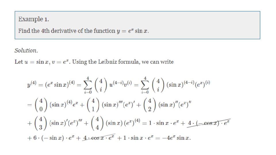
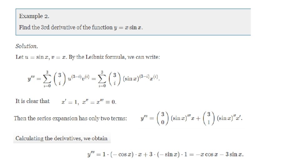
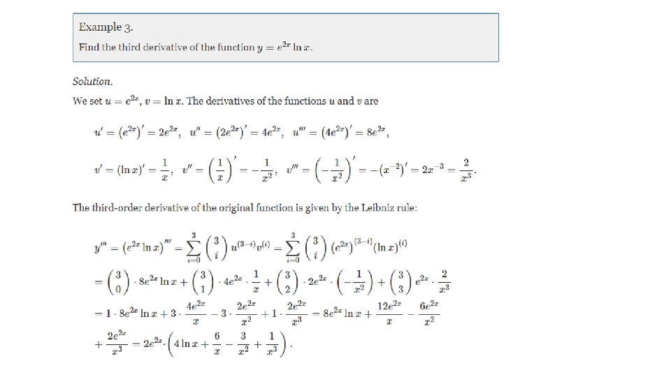
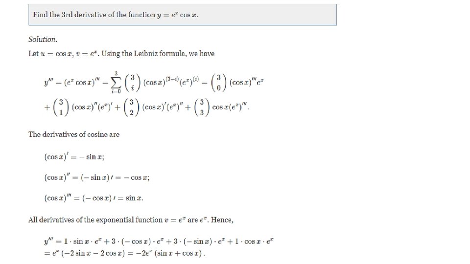
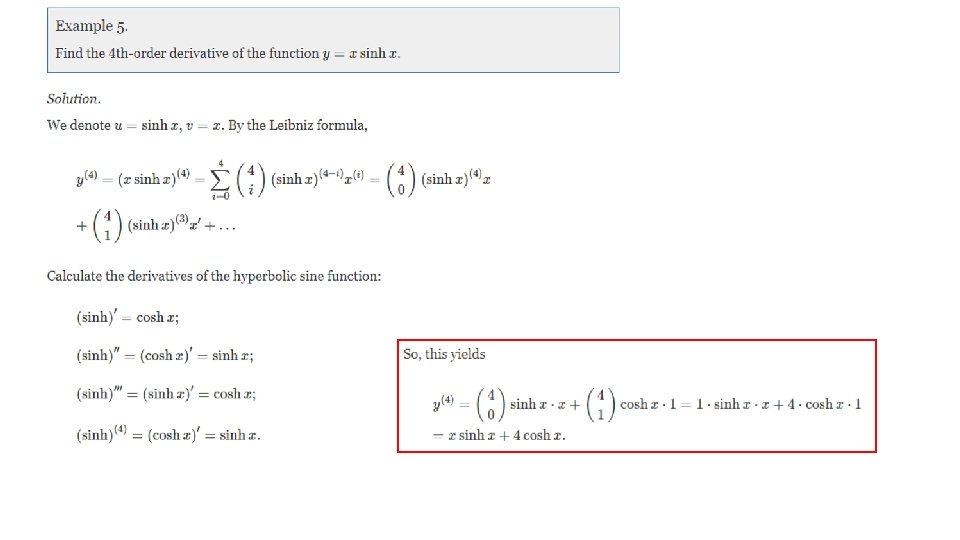
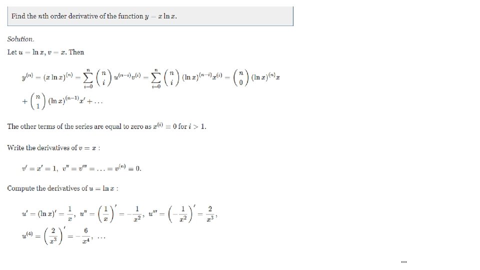
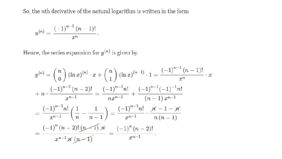
Leibniz Formula The Leibniz formula expresses the derivative on nth order of the product of two functions. Suppose that the functions u(x) and v(x) have the derivatives up to nth order. Consider the derivative of the product of these functions. The first derivative is described by the well known formula: Differentiating this expression again yields the second derivative:

Leibniz Formula where

Taylor’s Theorem n n If the function f and its first n+1 derivatives are continuous on an interval containing a and x, then the value of the function at x is given by where remainder Rn is defined as

Taylor’s Theorem Is the nth ordered Taylor polynomial.

Approximation with. Taylor polinomyals

Approximation with. Taylor polinomyals