Application Algorithms Lecture 17 Section 3 8 Wed

Application: Algorithms Lecture 17 Section 3. 8 Wed, Feb 9, 2005

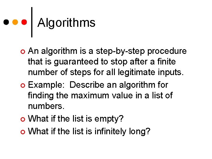
Algorithms An algorithm is a step-by-step procedure that is guaranteed to stop after a finite number of steps for all legitimate inputs. ¢ Example: Describe an algorithm for finding the maximum value in a list of numbers. ¢ What if the list is empty? ¢ What if the list is infinitely long? ¢

An Algorithmic Language An algorithmic language is much like a computer language. ¢ Its primary purpose is to express unambiguously the steps of an algorithm, including all decisions and special cases that may arise. ¢

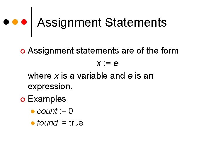
Assignment Statements Assignment statements are of the form x : = e where x is a variable and e is an expression. ¢ Examples ¢ count : = 0 l found : = true l

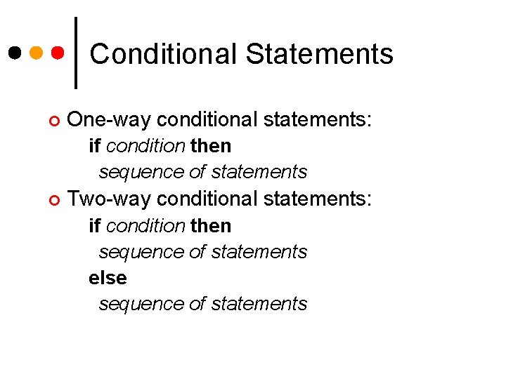
Conditional Statements ¢ One-way conditional statements: if condition then sequence of statements ¢ Two-way conditional statements: if condition then sequence of statements else sequence of statements

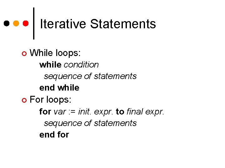
Iterative Statements ¢ While loops: while condition sequence of statements end while ¢ For loops: for var : = init. expr. to final expr. sequence of statements end for

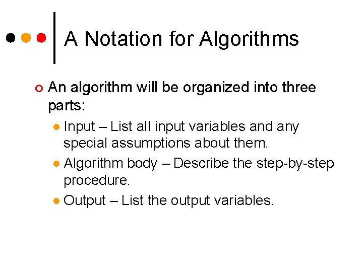
A Notation for Algorithms ¢ An algorithm will be organized into three parts: Input – List all input variables and any special assumptions about them. l Algorithm body – Describe the step-by-step procedure. l Output – List the output variables. l

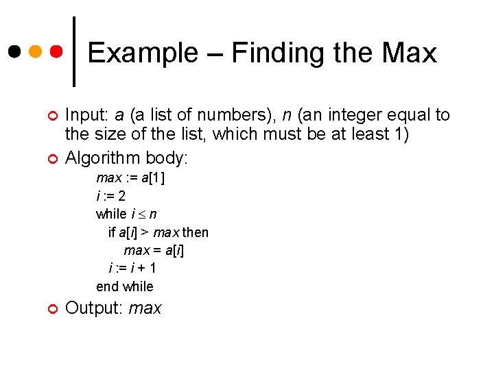
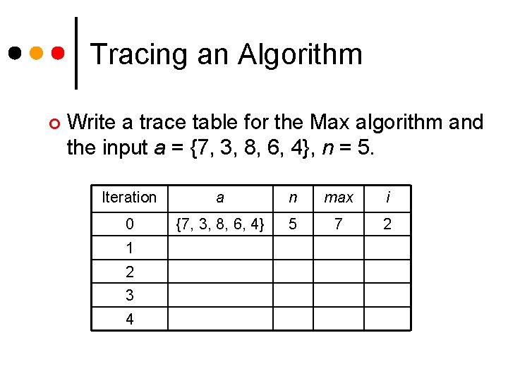
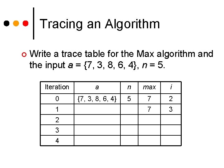
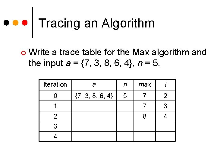
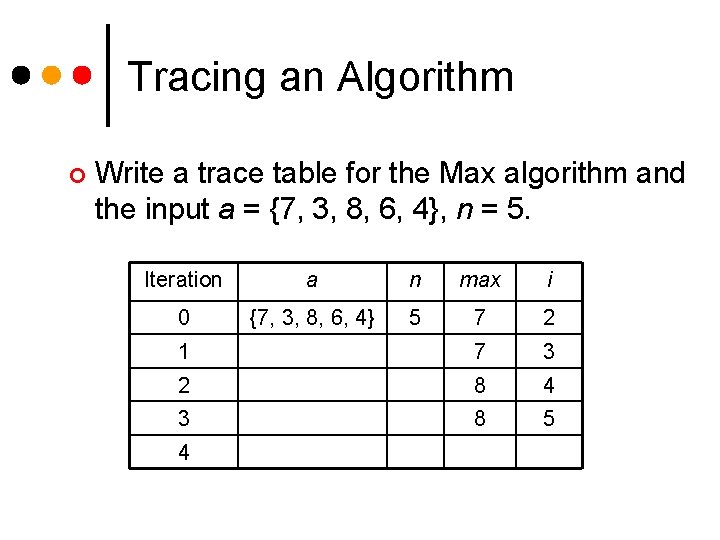
Example – Finding the Max ¢ ¢ Input: a (a list of numbers), n (an integer equal to the size of the list, which must be at least 1) Algorithm body: max : = a[1] i : = 2 while i n if a[i] > max then max = a[i] i : = i + 1 end while ¢ Output: max

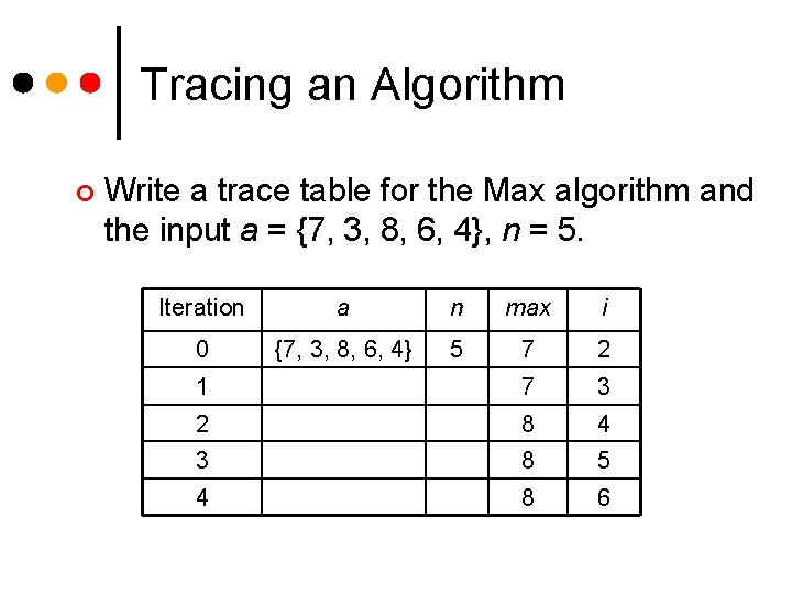
Tracing an Algorithm ¢ Write a trace table for the Max algorithm and the input a = {7, 3, 8, 6, 4}, n = 5. Iteration a n max i 0 {7, 3, 8, 6, 4} 5 7 2 1 2 3 4

Tracing an Algorithm ¢ Write a trace table for the Max algorithm and the input a = {7, 3, 8, 6, 4}, n = 5. Iteration a n max i 0 {7, 3, 8, 6, 4} 5 7 2 7 3 1 2 3 4

Tracing an Algorithm ¢ Write a trace table for the Max algorithm and the input a = {7, 3, 8, 6, 4}, n = 5. Iteration a n max i 0 {7, 3, 8, 6, 4} 5 7 2 1 7 3 2 8 4 3 4

Tracing an Algorithm ¢ Write a trace table for the Max algorithm and the input a = {7, 3, 8, 6, 4}, n = 5. Iteration a n max i 0 {7, 3, 8, 6, 4} 5 7 2 1 7 3 2 8 4 3 8 5 4

Tracing an Algorithm ¢ Write a trace table for the Max algorithm and the input a = {7, 3, 8, 6, 4}, n = 5. Iteration a n max i 0 {7, 3, 8, 6, 4} 5 7 2 1 7 3 2 8 4 3 8 5 4 8 6

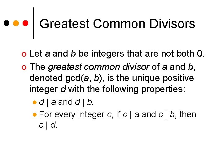
Greatest Common Divisors Let a and b be integers that are not both 0. ¢ The greatest common divisor of a and b, denoted gcd(a, b), is the unique positive integer d with the following properties: ¢ d | a and d | b. l For every integer c, if c | a and c | b, then c | d. l

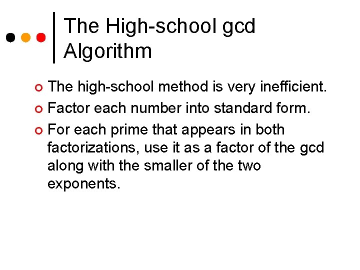
The High-school gcd Algorithm The high-school method is very inefficient. ¢ Factor each number into standard form. ¢ For each prime that appears in both factorizations, use it as a factor of the gcd along with the smaller of the two exponents. ¢

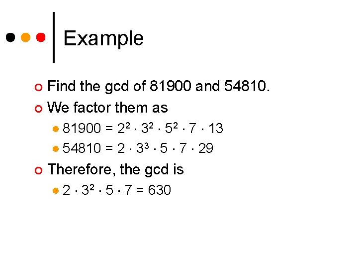
Example Find the gcd of 81900 and 54810. ¢ We factor them as ¢ 81900 = 22 32 52 7 13 l 54810 = 2 33 5 7 29 l ¢ Therefore, the gcd is l 2 32 5 7 = 630

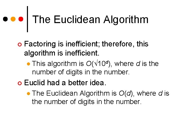
The Euclidean Algorithm ¢ Factoring is inefficient; therefore, this algorithm is inefficient. l ¢ This algorithm is O( 10 d), where d is the number of digits in the number. Euclid had a better idea. l The Euclidean Algorithm is O(d), where d is the number of digits in the number.

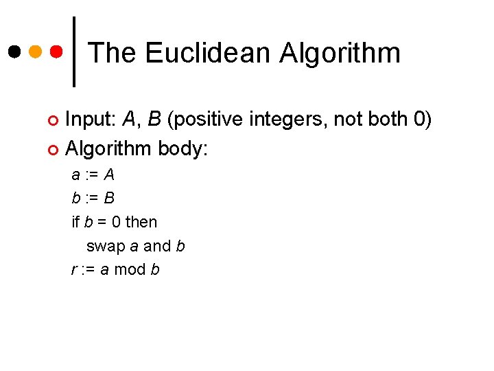
The Euclidean Algorithm Input: A, B (positive integers, not both 0) ¢ Algorithm body: ¢ a : = A b : = B if b = 0 then swap a and b r : = a mod b

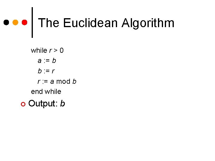
The Euclidean Algorithm while r > 0 a : = b b : = r r : = a mod b end while ¢ Output: b

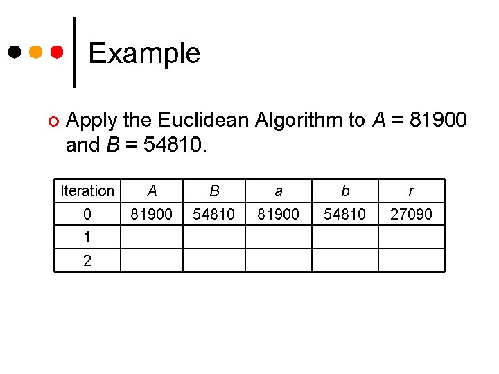
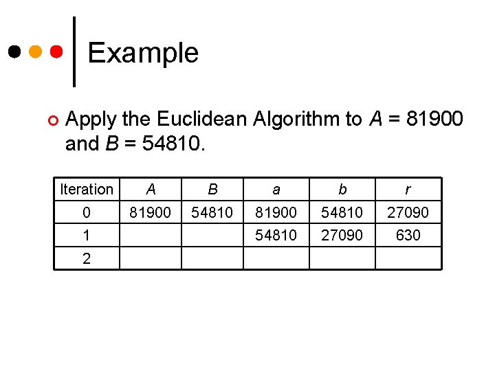
Example ¢ Apply the Euclidean Algorithm to A = 81900 and B = 54810. Iteration A B a b r 0 81900 54810 27090 1 2

Example ¢ Apply the Euclidean Algorithm to A = 81900 and B = 54810. Iteration A B a b r 0 81900 54810 27090 630 1 2

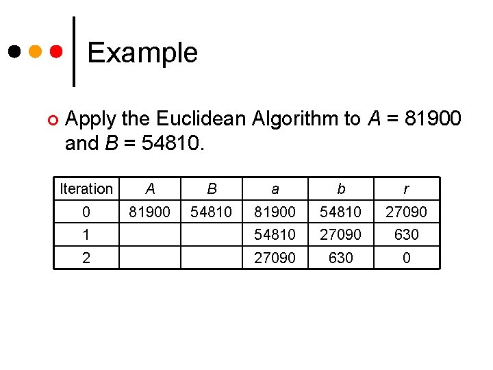
Example ¢ Apply the Euclidean Algorithm to A = 81900 and B = 54810. Iteration A B a b r 0 81900 54810 27090 1 54810 27090 630 2 27090 630 0

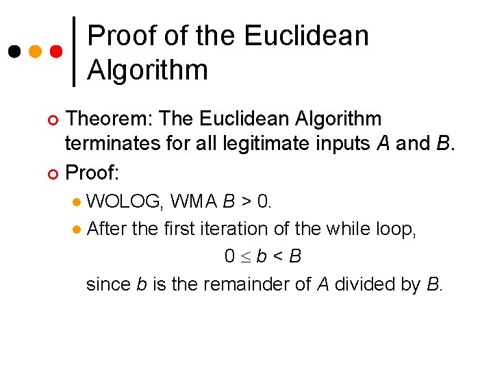
Proof of the Euclidean Algorithm Theorem: The Euclidean Algorithm terminates for all legitimate inputs A and B. ¢ Proof: ¢ WOLOG, WMA B > 0. l After the first iteration of the while loop, 0 b<B since b is the remainder of A divided by B. l

Proof Each iteration produces a nonnegative remainder that is smaller than the previous remainder. l This cannot happen more than B times before the remainder is 0. l

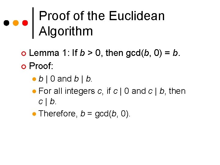
Proof of the Euclidean Algorithm Lemma 1: If b > 0, then gcd(b, 0) = b. ¢ Proof: ¢ b | 0 and b | b. l For all integers c, if c | 0 and c | b, then c | b. l Therefore, b = gcd(b, 0). l

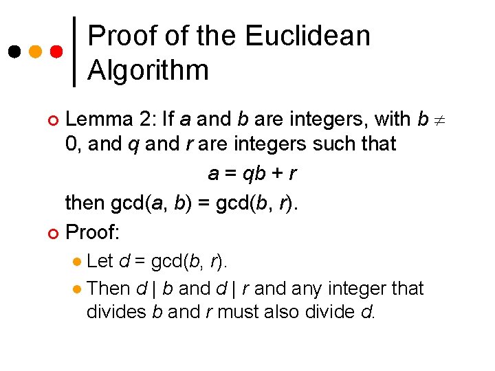
Proof of the Euclidean Algorithm Lemma 2: If a and b are integers, with b 0, and q and r are integers such that a = qb + r then gcd(a, b) = gcd(b, r). ¢ Proof: ¢ Let d = gcd(b, r). l Then d | b and d | r and any integer that divides b and r must also divide d. l

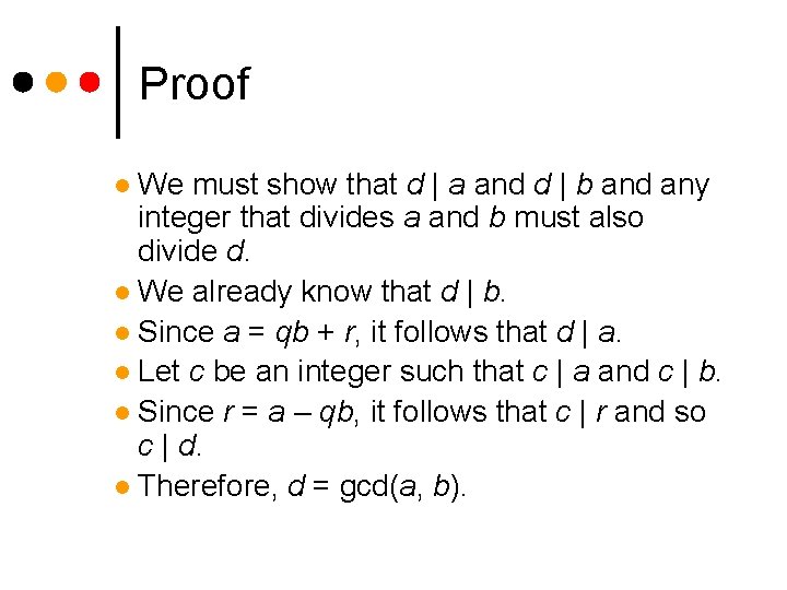
Proof We must show that d | a and d | b and any integer that divides a and b must also divide d. l We already know that d | b. l Since a = qb + r, it follows that d | a. l Let c be an integer such that c | a and c | b. l Since r = a – qb, it follows that c | r and so c | d. l Therefore, d = gcd(a, b). l

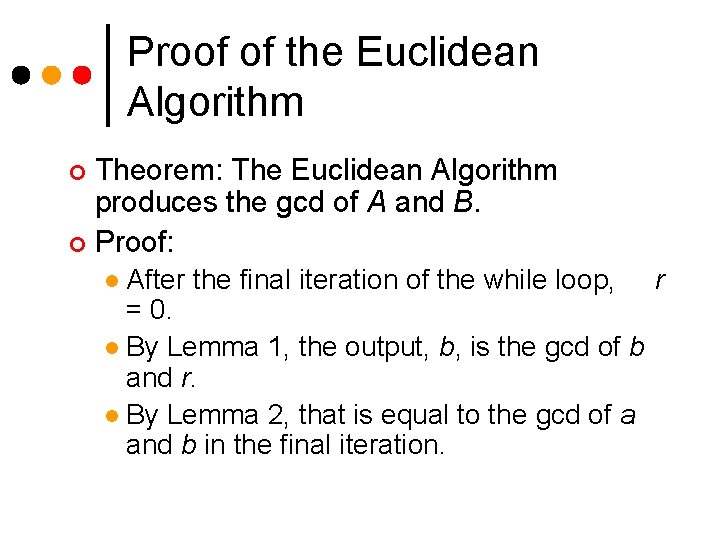
Proof of the Euclidean Algorithm Theorem: The Euclidean Algorithm produces the gcd of A and B. ¢ Proof: ¢ After the final iteration of the while loop, r = 0. l By Lemma 1, the output, b, is the gcd of b and r. l By Lemma 2, that is equal to the gcd of a and b in the final iteration. l

Proof But a and b on the last iteration were b and r on the previous iteration. l Therefore, gcd(a, b) on the last iteration equals gcd(b, r) on the previous iteration, which equals gcd(a, b) on the previous iteration, and so on. l Following this argument all the back to the first iteration, we see that the output is gcd(A, B). l

Proof In a later chapter, we will study mathematical induction. ¢ At that point, we will be able to make this argument more rigorous. ¢