Appendix to Chapter 1 Mathematics Used in Microeconomics

Appendix to Chapter 1 Mathematics Used in Microeconomics © 2004 Thomson Learning/South-Western

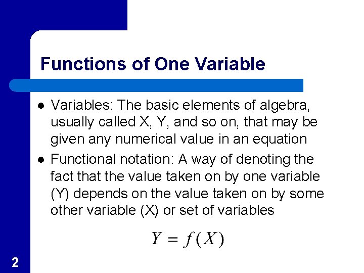
Functions of One Variable l l 2 Variables: The basic elements of algebra, usually called X, Y, and so on, that may be given any numerical value in an equation Functional notation: A way of denoting the fact that the value taken on by one variable (Y) depends on the value taken on by some other variable (X) or set of variables

Independent and Dependent Variables l l 3 Independent Variable: In an algebraic equation, a variable that is unaffected by the action of another variable and may be assigned any value Dependent Variable: In algebra, a variable whose value is determined by another variable or set of variables

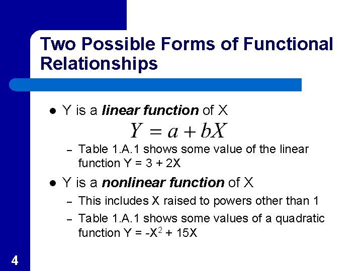
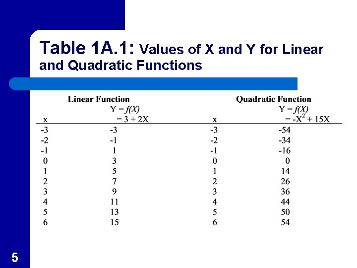
Two Possible Forms of Functional Relationships l Y is a linear function of X – l Y is a nonlinear function of X – – 4 Table 1. A. 1 shows some value of the linear function Y = 3 + 2 X This includes X raised to powers other than 1 Table 1. A. 1 shows some values of a quadratic function Y = -X 2 + 15 X

Table 1 A. 1: Values of X and Y for Linear and Quadratic Functions 5

Graphing Functions of One Variable l l Graphs are used to show the relationship between two variables Usually the dependent variable (Y) is shown on the vertical axis and the independent variable (X) is shown on the horizontal axis – 6 However, on supply and demand curves, this approach is reversed

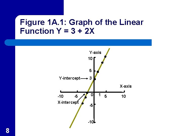
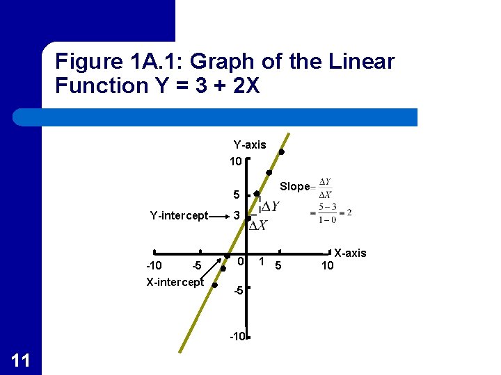
Linear Function l l l 7 A linear function is an equation that is represented by a straight-line graph Figure 1 A. 1 represents the linear function Y=3+2 X As shown in Figure 1 A. 1, linear functions may take on both positive and negative values

Figure 1 A. 1: Graph of the Linear Function Y = 3 + 2 X Y-axis 10 5 Y-intercept 3 X-axis -10 -5 X-intercept 0 -5 -10 8 1 5 10

Intercept l l The general form of a linear equation is Y = a + b. X The Y-intercept is the value of Y when X equals 0 – 9 Using the general form, when X = 0, Y = a, so this is the intercept of the equation

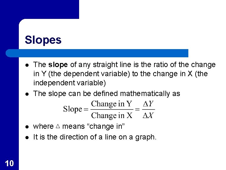
Slopes l l 10 The slope of any straight line is the ratio of the change in Y (the dependent variable) to the change in X (the independent variable) The slope can be defined mathematically as where means “change in” It is the direction of a line on a graph.

Figure 1 A. 1: Graph of the Linear Function Y = 3 + 2 X Y-axis 10 5 Y-intercept -10 -5 X-intercept 3 0 -5 -10 11 Slope 1 5 X-axis 10

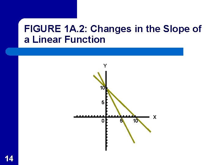
Slopes l l 12 The slope is the same along a straight line. For the general form of the linear equation the slope equals b The slope can be positive (as in Figure 1 A. 1), negative (as in Figure 1 A. 2) or zero If the slope is zero, the straight line is horizontal with Y = intercept

Changes in Slope l l l 13 In economics we are often interested in changes in the parameters (a and b of the general linear equation) In Figure 1 A. 2 the (negative) slope is doubled while the intercept is held constant In general, a change in the slope of a function will cause rotation of the function without changing the intercept

FIGURE 1 A. 2: Changes in the Slope of a Linear Function Y 10 5 0 14 5 10 X

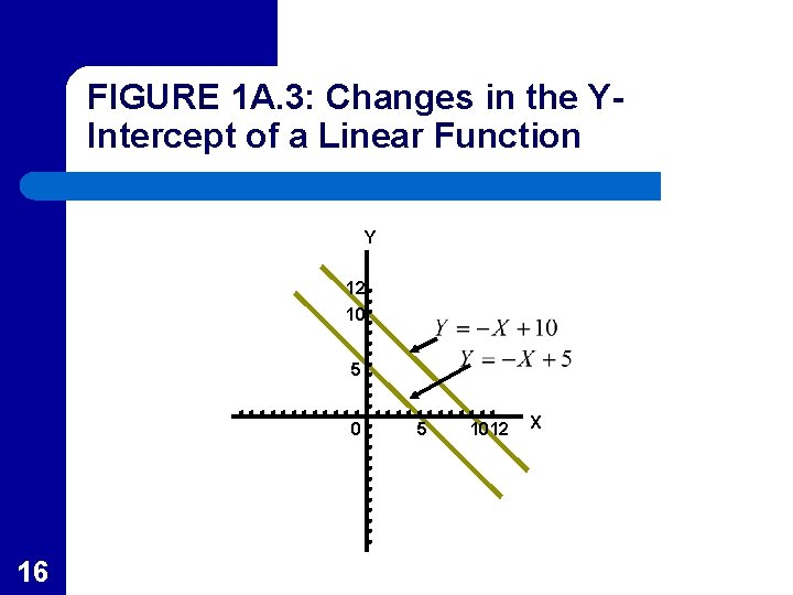
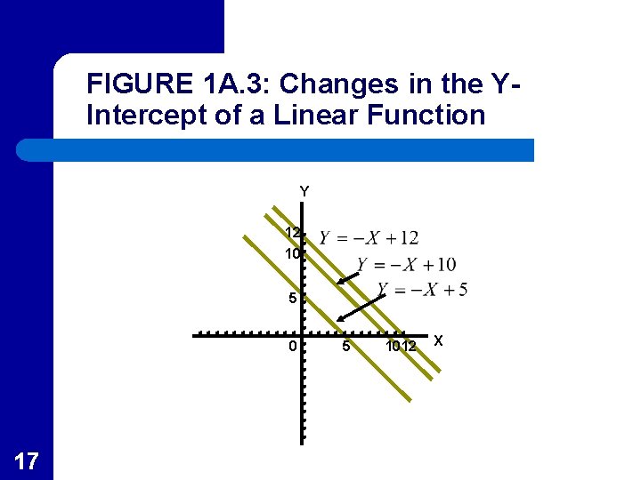
Changes in Intercept l l When the slope is held constant but the intercept is changed in a linear function, this results in parallel shifts in the function In Figure 1 A. 3, the slope of all three functions is -1, but the intercept equals 5 for the line closest to the origin, increases to 10 for the second line and 12 for the third – 15 These represent “Shifts” in a linear function.

FIGURE 1 A. 3: Changes in the YIntercept of a Linear Function Y 12 10 5 0 16 5 1012 X

FIGURE 1 A. 3: Changes in the YIntercept of a Linear Function Y 12 10 5 0 17 5 1012 X

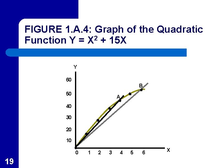
Nonlinear Functions l l l 18 Figure 1 A. 4 shows the graph of the nonlinear function Y = -X 2 + 15 X As the graph shows, the slope of the line is not constant but, in this case, diminishes as X increases This results in a concave graph which could reflect the principle of diminishing returns

FIGURE 1. A. 4: Graph of the Quadratic Function Y = X 2 + 15 X Y 60 B 50 A 40 30 20 10 0 19 1 2 3 4 5 6 X

The Slope of a Nonlinear Function l l l 20 The graph of a nonlinear function is not a straight line Therefore it does not have the same slope at every point The slope of a nonlinear function at a particular point is defined as the slope of the straight line that is tangent to the function at that point.

Marginal Effects l l 21 The marginal effect is the change in Y brought about by one unit change in X at a particular value of X (Also the slope of the function) For a linear function this will be constant, but for a nonlinear function it will vary from point to point

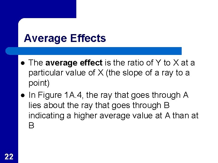
Average Effects l l 22 The average effect is the ratio of Y to X at a particular value of X (the slope of a ray to a point) In Figure 1 A. 4, the ray that goes through A lies about the ray that goes through B indicating a higher average value at A than at B

Calculus and Marginalism l l l 23 In graphical terms, the derivative of a function and its slope are the same concept Both provide a measure of the marginal inpact of X on Y Derivatives provide a convenient way of studying marginal effects.

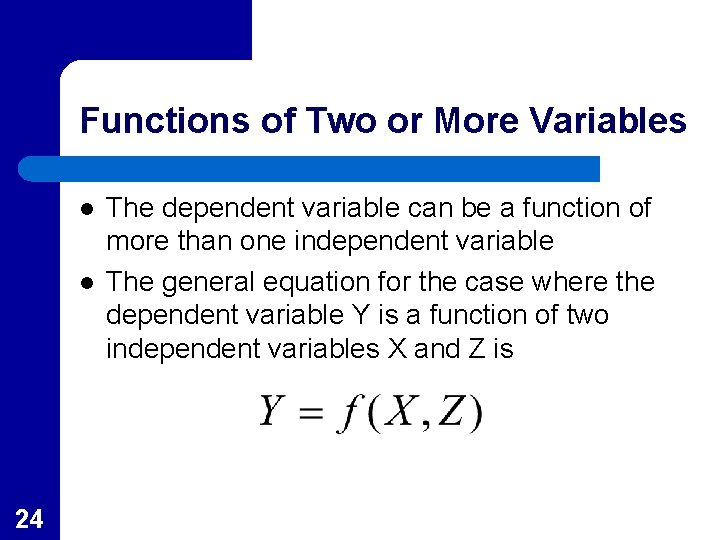
Functions of Two or More Variables l l 24 The dependent variable can be a function of more than one independent variable The general equation for the case where the dependent variable Y is a function of two independent variables X and Z is

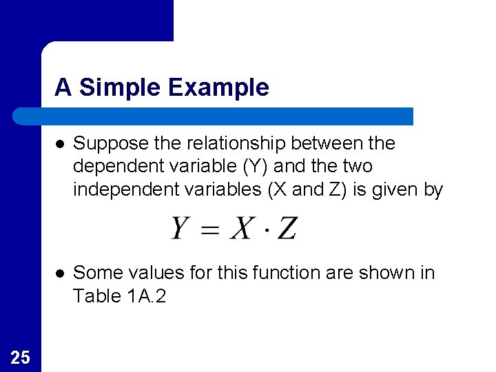
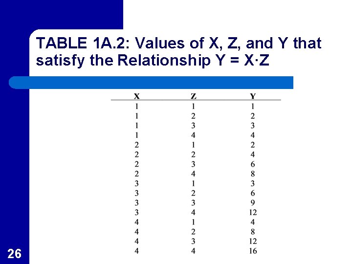
A Simple Example 25 l Suppose the relationship between the dependent variable (Y) and the two independent variables (X and Z) is given by l Some values for this function are shown in Table 1 A. 2

TABLE 1 A. 2: Values of X, Z, and Y that satisfy the Relationship Y = X·Z 26

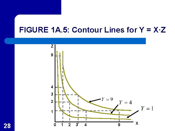
Graphing Functions of Two Variables l l l 27 Contour lines are frequently used to graph functions with two independent variables Contour lines are lines in two dimensions that show the sets of values of the independent variables that yield the same value for the dependent variable Contour lines for the equation Y = X·Z are shown in Figure 1 A. 5

FIGURE 1 A. 5: Contour Lines for Y = X·Z Z 9 4 3 2 1 28 0 1 2 3 4 9 X

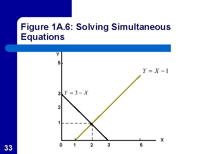
Simultaneous Equations l l 29 These are a set of equations with more than one variable that must be solved together for a particular solution When two variables, say X and Y, are related by two different equations, it is sometime possible to solve these equations to get a set of values for X and Y that satisfy both equations

Simultaneous Equations The equations [1 A. 17] can be solved for the unique solution 30

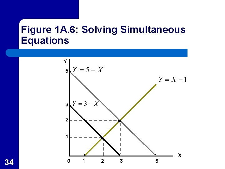
Changing Solutions for Simultaneous Equations The equations [1 A. 19] can be solved for the unique solution 31

Graphing Simultaneous Equations l l l 32 The two simultaneous equations systems, 1 A. 17 and 1 A. 19 are graphed in Figure 1 A. 6 The intersection of the graphs of the equations show the solutions to the equations systems These graphs are very similar to supply and demand graphs

Figure 1 A. 6: Solving Simultaneous Equations Y 5 3 2 1 X 33 0 1 2 3 5

Figure 1 A. 6: Solving Simultaneous Equations Y 5 3 2 1 X 34 0 1 2 3 5

Empirical Microeconomics and Econometrics l l l Economists test the validity of their models by looking at data from the real world Econometrics is used for this purpose Two important aspects of econometrics are – – 35 random influences the ceteris paribus assumption

Random Influences l l l 36 No economic model exhibits perfect accuracy so actual price and quantity values will be scattered around the “true” demand curve Figure 1 A. 7 shows the unknown true demand curve and the actual points observed in the data from the real world The problem is to infer the true demand curve

FIGURE 1 A. 7: Inferring the Demand Curve from Real-World Data Price (P) D Quantity (Q) 37

Random Influences l l 38 Technically, the problem is statistical inference: the use of actual data and statistical techniques to determine quantitative economic relationships Since no single straight line will fit all of the data points, the researcher must give careful consideration to the random influences to get the best line possible

The Ceteris Paribus Assumption l To control for the “other things equal” assumption two things must be done – – l 39 Data should be collected on all of the other factors that affect demand, and appropriate procedures must be used to control for these measurable factors in the analysis Generally the researcher has to make some compromises which leads to many controversies in testing economic models