Appendix II Probability Theory Refresher Leonard Kleinrock Queueing

Appendix II – Probability Theory Refresher Leonard Kleinrock, Queueing Systems, Vol I: Theory Nelson Fonseca, State University of Campinas, Brazil

Appendix II – Probability Theory Refresher

• Random event: statistical regularity • Example: If one were to toss a fair coin four times, one expects on the average two heads and two tails. There is one chance in sixteen that 88 no heads will occur. If we tossed the coin a million times, the odds are better than 10 to 1 that at least 490. 000 heads will occur.

II. 1 Rules of the game • Real-world experiments: – A set of possible experimental outcomes – A grouping of these outcomes into classes called results – The relative frequency of these classes in many independent trials of the experiment Frequency = number of times the experimental outcome falls into that class, divided by number of times the experiment is performed

• Mathematical model: three quantities of interest that are in one-to-one relation with the three quantities of experimental world 1. A sample space is a collection of objects that corresponds to the set of mutually exclusive exhaustive outcomes of the model of an experiment. Each object is in the set S is referred to as a sample point 2. A family of events denoted {A, B, C, …}in which each event is a set of samples points { }
 of the events defined")
3. A probability measure P which is an assignment (mapping) of the events defined on S into the set of real numbers. The notation is P[A], and have these mapping properties: a) For any event A, 0 <= P[A] <=1 (II. 1) b) P[S]=1 (II. 2) c) If A and B are “mutually exclusive” events then P[A U B]=P[A]+P[B] (II. 3)

• Notation • Exhaustive set of events: a set of events whose union forms the sample space S • Set of mutually exclusive exhaustive events , which have the properties
 along with Axioms (II. 2)(II. 3) form")
• The triplet (S, , P) along with Axioms (II. 2)(II. 3) form a probability system • Conditional probability • The event B forces us to restrict attention from the original sample space S to a new sample space defined by the event B, since B must now have a total probability of unity. We magnify the probabilities associated with conditional events by dividing by the term P[B]

• Two events A, B are said to be statistically independent if and only if • If A and B are independent • Theorem of total probability If the event B is to occur it must occur in conjunction with exactly one of the mutually exclusive exhaustive events Ai

• The second important form of theorem of total probability • Instead of calculating the probability of some complex event B, we calculate the occurrence of this event with mutually exclusive events

• Bayes’ theorem i Where {A }are a set of events mutually exclusive and exhaustive • Example: You have just entered a casino and gamble with a twin brother, one is honest and the other not. You know that you lose with probability=½ if you play with the honest brother, and lose with probability=P if you play with the cheating brother

II. 2 Random variables • Random variable is a variable whose value depends upon the outcome of a random experiment • To each outcome, we associate a real number, which is in fact the value the random variable takes on that outcome • Random variable is a mapping from the points of the sample space into the (real) line

• Example: If we win the game we win $5, if we lose we win -$5 and if we draw we win S $0. W (3/8) D L (1/4) (3/8)
, also known as the cumulative distribution function")
• Probability distribution function (PDF), also known as the cumulative distribution function

1 -5 0 +5 x
 • The pdf integrated over an interval gives")
• Probability density function (pdf) • The pdf integrated over an interval gives the probability that the random variable X lies in that interval

• Distributed random variable -5 0 +5
 – Functions of more than one variable – “Marginal”")
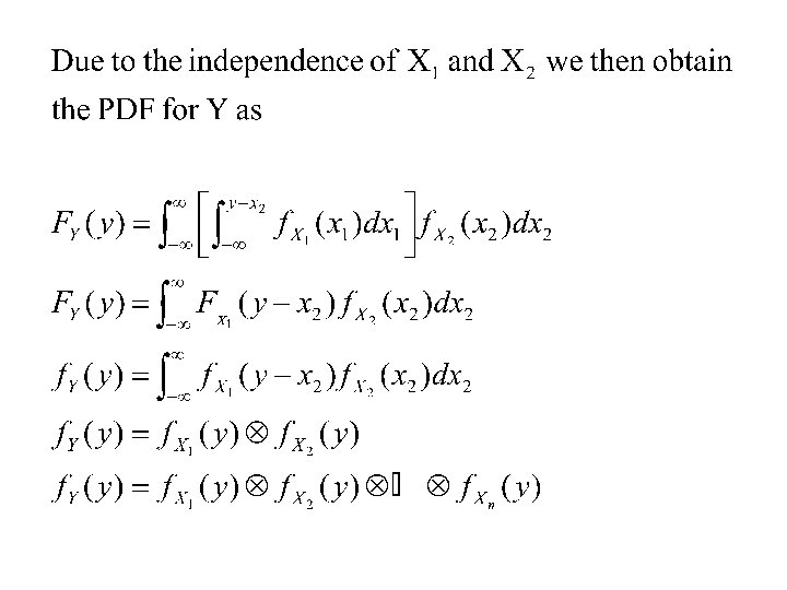
• Impulse function (discontinuous) – Functions of more than one variable – “Marginal” density function – Two random variables X and Y are said to be independent if and only if

• We can define conditional distributions and densities • Function of one random variable • Given the random variable X and its PDF, one should be able to calculate the PDF for the variable Y

y y 0

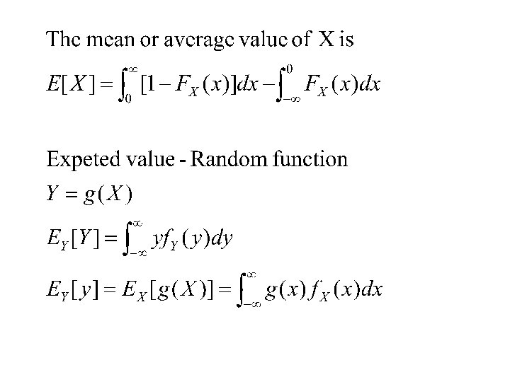
II. 3 Expectation • Stieltjes integrals deal with discontinuities and impulses Let

• The Stieltjes integral will always exist and therefore it avoids the issue of impulses • Without impulses the pdf may not exist • When impulses are permitted we have

• Expectation of the sum of two random variables

• The expectation of the sum of two random variables is always equal to the sum of the expectations of each variable • This is true even if the variables are dependent • The expectation operator is a linear operator

The question is: what is the probability of your being playing with the cheating brother since you lost?

– The expected result of the product of variables is equal to the product of the expected values if the variables are independent – Expected value of the product of random functions

– nth moment – nth central moment

– The nth central moment can be expressed as a function of n moments – First central moment = 0
 – Coefficient of")
– Second central moment => variance – Standard deviation (central moment) – Coefficient of variation

Pareto Notation Range Parameters – Scale Parameters – Shape

Pareto Distribution Function

Pareto Probability Density Function

Pareto a=1 b=1 a=1 b=2

Pareto a=10 b=5 a=5 b=10

a=5 b=10 Pareto

Pareto Expected Value

Pareto Moments Uncentered

Weibull Notation Range Parameters – Scale Parameters – Shape

Weibull Probability Density Function

Weibull Distribution Function

Weibull b=1 c=1 b=2 c=1

Weibull b=1 c=2 b=2 c=2

Weibull b=10 c=5 b=5 c=10

b=25 c=10 Weibull

Weibull Moments Uncentered

Weibull Expected Value

Weibull Variance

Lognormal Notation Range Parameters – Scale Parameters – Shape

Lognormal Probability Density Function

Lognormal Expected Value

Lognormal Variance

Lognormal m=0 s=0. 5 m=0 s=0. 7

Lognormal m=1 s=0. 5 m=1 s=0. 7

Lognormal m=0 s=0. 1 m=1 s=0. 1

Lognormal m=0 s=1 m=1 s=1

m=0 s=1 Lognormal

Normal Notation Range Parameters – Scale Parameters – Shape

Normal Probability Density Function

Normal m=10 s=2 m=10 s=1

Normal m=0 s=2 m=0 s=1

m=0 s=1 Normal

Normal Expected Value

Normal Variance

Exponential Probability Density Function Distribution Function

II. 4 Transforms, generating functions and characteristic function • Characteristic function of a random variable x(f. X(u)) is given by: – u – real variable

– Expanding ejux and integrating

– Notation

– Moment generation function

• Laplace transform of the pdf – Notation:

– Example

– Probability generating function – discrete variable

– Sum of n independent variables – xi – Identically distributed

– Sum of independent variables

– x 1 and x 2 independent – The variance of the sum of independent random variables is equal to the sum of variances

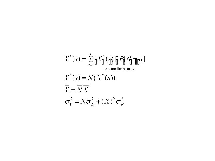
– Variable sum of independent variables and the number of variables is a random variable – Where N: is a random variable with mean N and variance s. X 2 – [ Xi ] is independent and identically distributed – N and [ Xi ] independent – FY(y) - Compound distribution
![– [ Xi ] - identically distributed variables](http://slidetodoc.com/presentation_image_h/0ae2701f13881c8afcaa79d8c229b178/image-78.jpg "– [ Xi ] - identically distributed variables")
– [ Xi ] - identically distributed variables

II. 6. Stochastic process – To each point of the sample process space wÎS a time function x is associated => Stochastic process family

– Autocorrelation: – Wide sense stationary process
- Slides: 81