Appendix 4 A A Formal Model of Consumption

Appendix 4. A A Formal Model of Consumption and Saving Micro-foundation of Macro Abel & Bernake: Macro Ch 3 Varian: Micro Ch 10 1

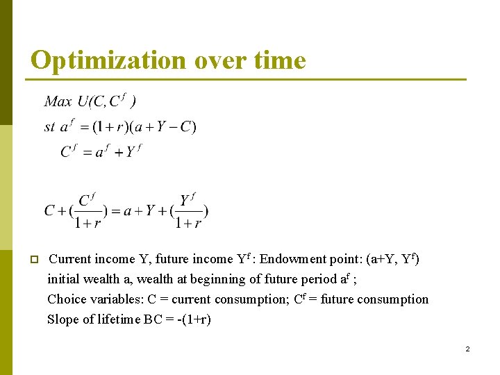
Optimization over time p Current income Y, future income Yf : Endowment point: (a+Y, Yf) initial wealth a, wealth at beginning of future period af ; Choice variables: C = current consumption; Cf = future consumption Slope of lifetime BC = -(1+r) 2

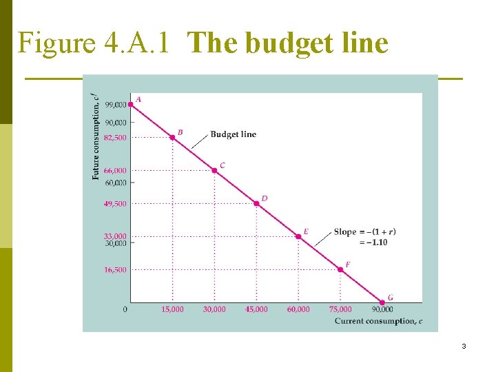
Figure 4. A. 1 The budget line 3

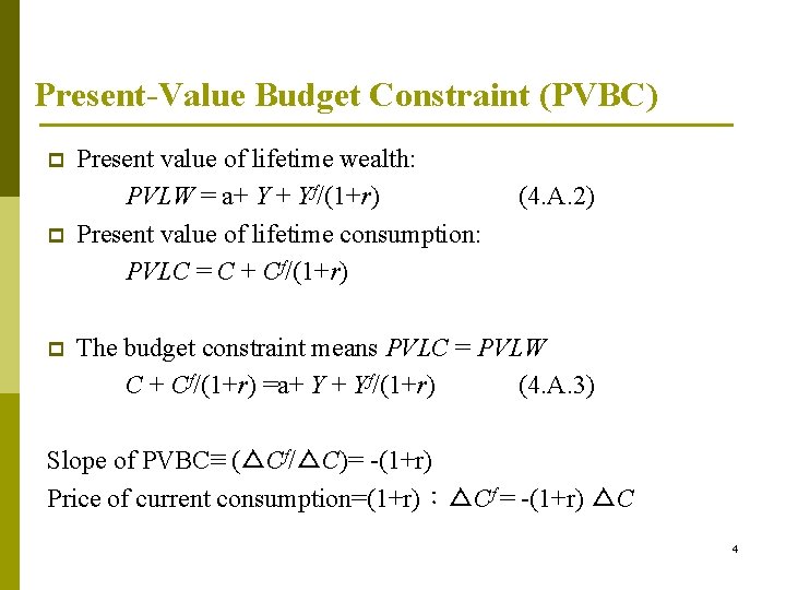
Present-Value Budget Constraint (PVBC) p p p Present value of lifetime wealth: PVLW = a+ Y + Yf/(1+r) Present value of lifetime consumption: PVLC = C + Cf/(1+r) (4. A. 2) The budget constraint means PVLC = PVLW C + Cf/(1+r) =a+ Y + Yf/(1+r) (4. A. 3) Slope of PVBC≡ (△Cf/△C)= -(1+r) Price of current consumption=(1+r)：△Cf = -(1+r) △C 4

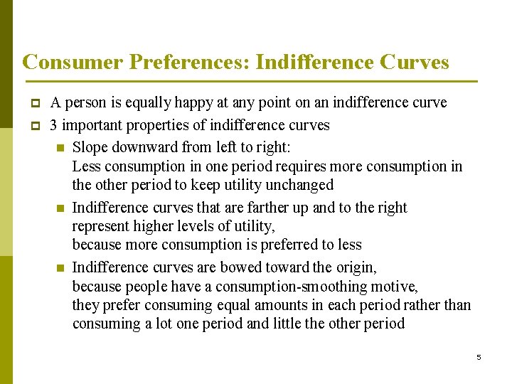
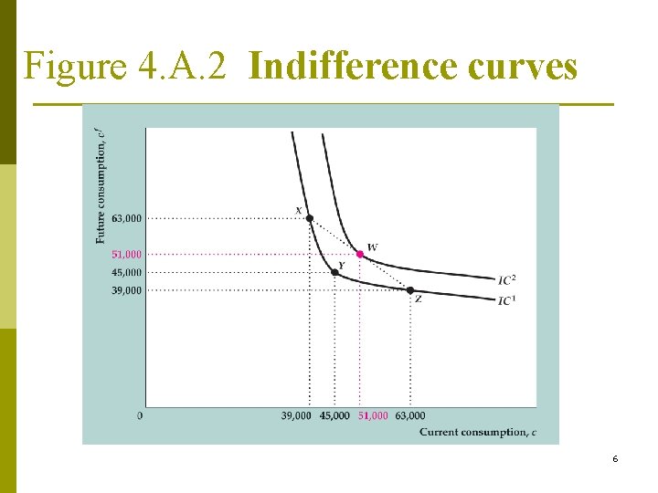
Consumer Preferences: Indifference Curves p p A person is equally happy at any point on an indifference curve 3 important properties of indifference curves n Slope downward from left to right: Less consumption in one period requires more consumption in the other period to keep utility unchanged n Indifference curves that are farther up and to the right represent higher levels of utility, because more consumption is preferred to less n Indifference curves are bowed toward the origin, because people have a consumption-smoothing motive, they prefer consuming equal amounts in each period rather than consuming a lot one period and little the other period 5

Figure 4. A. 2 Indifference curves 6

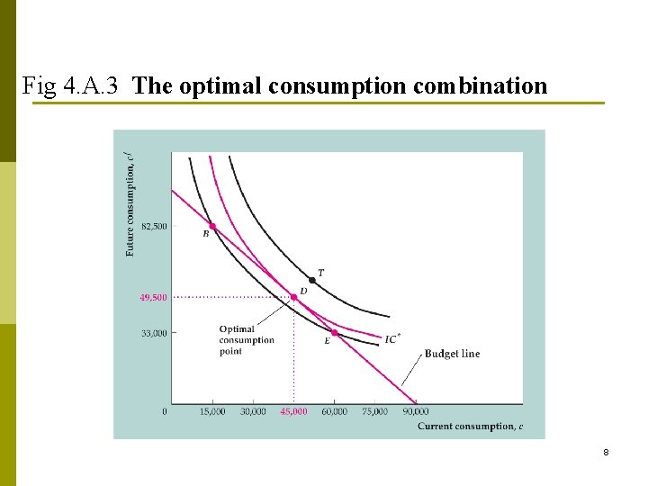
The Optimal Level of Consumption p Optimal consumption point: the budget line is tangent to an indifference curve (Fig. 4. A. 3) Tangency condition: ? 7

Fig 4. A. 3 The optimal consumption combination 8

Saving (S), a lender or a borrower p S≡Y-C If C=Y, S=0 If C<Y, S>0 If C>Y, S<0 p a f= 0, C=a+Y: no-borrowing, no-lending af>0, C< a+Y: lender, with interest income af< 0, C< a+Y: borrower, with interest payment 9

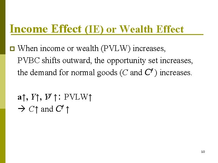
Income Effect (IE) or Wealth Effect p When income or wealth (PVLW) increases, PVBC shifts outward, the opportunity set increases, the demand for normal goods (C and Cf ) increases. a↑, Yf ↑: PVLW↑ C↑ and Cf ↑ 10

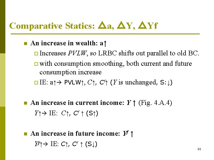
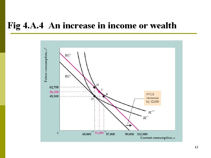
Comparative Statics: △a, △Yf n An increase in wealth: a↑ p Increases PVLW, so LRBC shifts out parallel to old BC. p with consumption smoothing, both current and future consumption increase p IE: a↑ PVLW↑, Cf↑ (Y is unchanged, S: ↓) n An increase in current income: Y ↑ (Fig. 4. A. 4) Y↑ IE: C↑, Cf ↑ (S↑) n An increase in future income: Yf ↑ Yf↑ IE: C↑, Cf ↑ (S↓) 11

Fig 4. A. 4 An increase in income or wealth 12

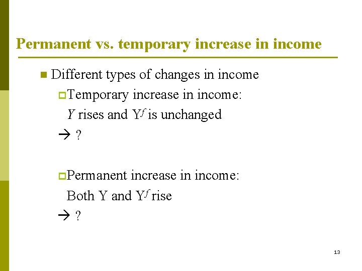
Permanent vs. temporary increase in income n Different types of changes in income p Temporary increase in income: Y rises and Yf is unchanged ? p Permanent increase in income: Both Y and Yf rise ? 13

The permanent income theory n This distinction made by Milton Friedman in the 1950 s and is known as the permanent income theory p Permanent changes in income lead to much larger changes in consumption p Thus permanent income changes are mostly consumed, while temporary income changes are mostly saved 14

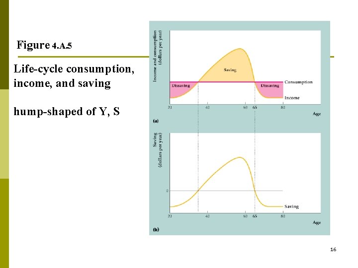
Life-Cycle Model p p p developed by Franco Modigliani and associates in the 1950 s n Patterns of income, consumption, and saving over an individual’s lifetime (Fig. 4. A. 5) Real income steadily rises over time until near retirement; at retirement, income drops sharply Lifetime pattern of consumption is much smoother than the income pattern. 15

Figure 4. A. 5 Life-cycle consumption, income, and saving hump-shaped of Y, S 16

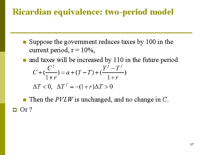
Ricardian equivalence: two-period model n n Suppose the government reduces taxes by 100 in the current period, r = 10%, and taxes will be increased by 110 in the future period Then the PVLW is unchanged, and no change in C. Or ? n p 17

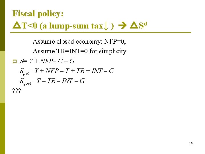
Fiscal policy: △T<0 (a lump-sum tax↓ ) △Sd Assume closed economy: NFP=0, Assume TR=INT=0 for simplicity p S= Y + NFP– C – G Spvt= Y + NFP – T + TR + INT – C Sgovt =T – TR – INT – G ? ? ? 18

Fiscal policy: △G>0 △Sd 19

Excess sensitivity of consumption p Generally, life cycle or permanent income theory have been supported by looking at real-world data n But data shows some excess sensitivity of consumption to changes in current income p This could be due to short-sighted behavior p Or it could be due to borrowing constraints 20

Borrowing constraints n n n If a person wants to borrow and can’t, the borrowing constraint is binding A consumer with a binding borrowing constraint spends all income and wealth on consumption. p So an increase in income or wealth will be entirely spent on consumption as well p This causes consumption to be excessively sensitive to current income changes Perhaps 20% to 50% of the U. S. population faces binding borrowing constraints. 21

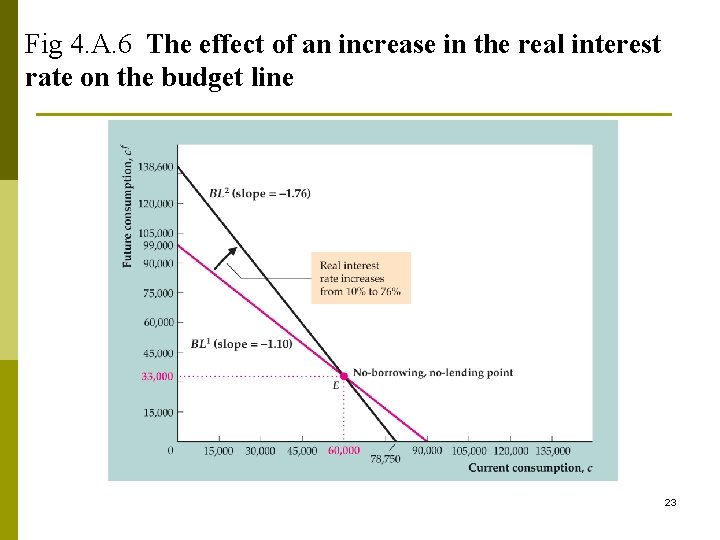
Comparative statics: change in r p r↑(Fig. 4. A. 6) n n one point on the old BC is also on the new BC: the no-borrowing, no-lending point Slope of new budget line is steeper 22

Fig 4. A. 6 The effect of an increase in the real interest rate on the budget line 23

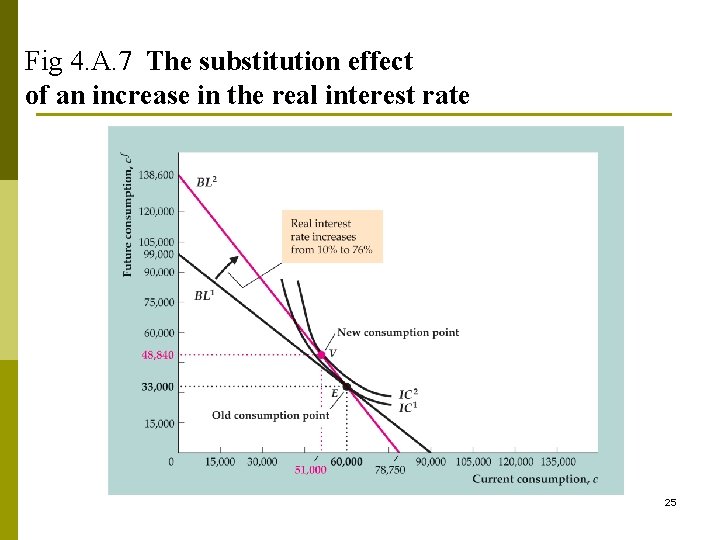
Intertemporal substitution effect (ISE) r↑makes future consumption cheaper relative to current consumption n use cheaper Cf to substitute more costly C, C↓(S↑), Cf ↑ n 24

Fig 4. A. 7 The substitution effect of an increase in the real interest rate 25

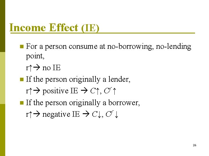
Income Effect (IE) For a person consume at no-borrowing, no-lending point, r↑ no IE n If the person originally a lender, r↑ positive IE C↑, Cf ↑ n If the person originally a borrower, r↑ negative IE C↓, Cf ↓ n 26

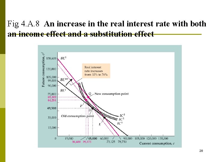
Δr: Total effect =ISE +IE p IE and ISE together n If a person consumes at no-borrowing, no-lending point (Fig. 4. A. 7), ? n For a lender, (Fig. 4. A. 8) ? n For a borrower, ? 27

Fig 4. A. 8 An increase in the real interest rate with both an income effect and a substitution effect 28

Δr aggregate saving n The effect on aggregate saving of r↑ is ambiguous theoretically. p Empirical research suggests that saving ↑ (Saving function is positively-sloped) p But the effect is small 29

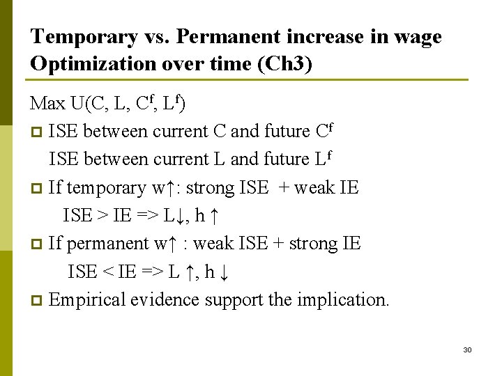
Temporary vs. Permanent increase in wage Optimization over time (Ch 3) Max U(C, L, Cf, Lf) p ISE between current C and future Cf ISE between current L and future Lf p If temporary w↑: strong ISE + weak IE ISE > IE => L↓, h ↑ p If permanent w↑ : weak ISE + strong IE ISE < IE => L ↑, h ↓ p Empirical evidence support the implication. 30