AP STATISTICS Chapter 3 Scatterplots and Correlation Size

AP STATISTICS Chapter 3: Scatterplots and Correlation

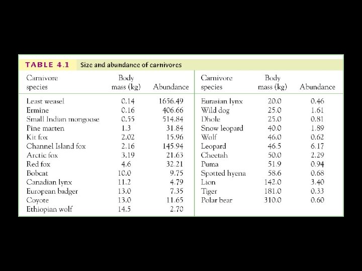
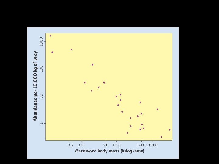
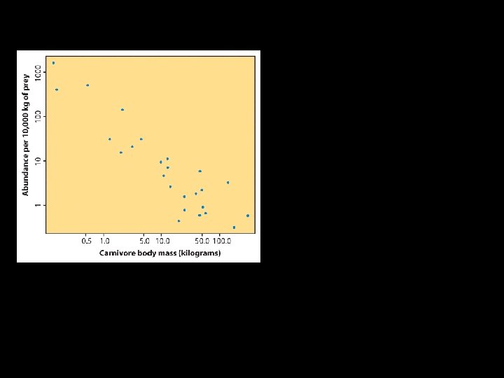
Size and abundance of carnivores

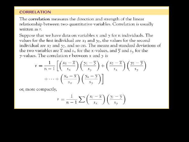
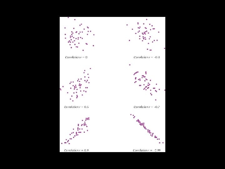
Basically r tells us the strength and direction of two variables

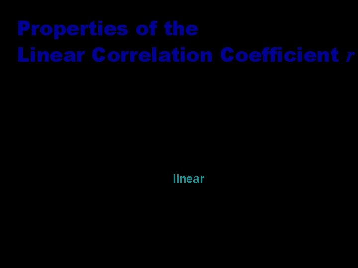
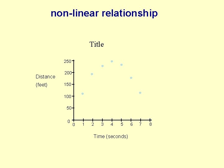
Properties of the Linear Correlation Coefficient r • 1. – 1 £ r £ 1 • 2. Value of r does not change if all values of either variable are converted to a different scale • 3. Interchanging all x and y values will not change r • 4. r measures strength of a linear relationship • 5. No linear relationship does not imply no relationship at all. There is a possibility of a non-linear relationship.

non-linear relationship Title 250 Distance (feet) 200 150 100 50 0 0 1 2 3 4 5 Time (seconds) 6 7 8

Abundance of carnivores Correlation tells us about strength (scatter) and direction of the linear relationship between two quantitative variables. R does not change when we change units of measurement. R is not resistant and is strongly affected by outliers In addition, we would like to have a numerical description of how both variables vary together. For instance, is one variable increasing faster than the other one? And we would like to make predictions based on that numerical description.

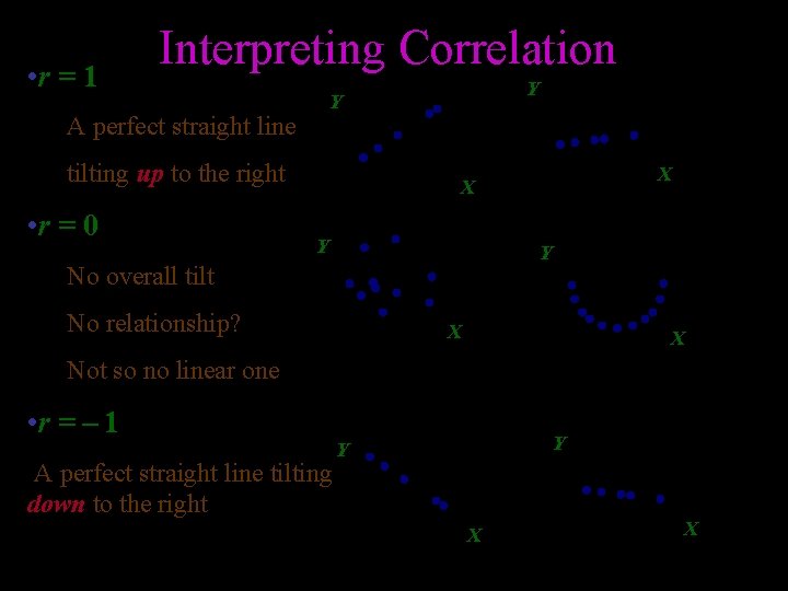
• r = 1 Interpreting Correlation Y Y A perfect straight line tilting up to the right • r = 0 X X Y Y No overall tilt No relationship? X X Not so no linear one • r = – 1 A perfect straight line tilting down to the right Y Y X X

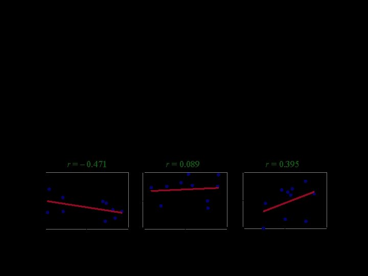
No Correlation r = – 0. 471 Nonlinear Correlation r = 0. 089 r = 0. 395

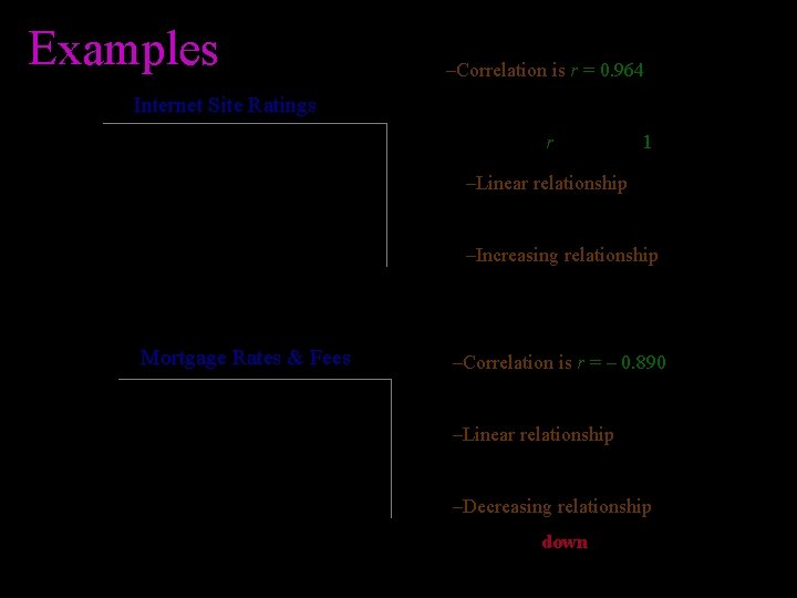
Minutes person Examples –Correlation is r = 0. 964 Internet Site Ratings 90 • (since r is close to 1) e. Bay Yahoo! 60 –Linear relationship MSN 30 0 • Very strong positive association • Straight line with scatter –Increasing relationship 0 100 Pages person 200 Mortgage Rates & Fees –Correlation is r = – 0. 890 Interest rate 6. 0% • Strong negative association –Linear relationship 5. 5% 5. 0% 0% • Tilts up and to the right positive • Straight line with scatter –Decreasing relationship 1% 2% Loan fee 3% 4% • Tilts down and to the right

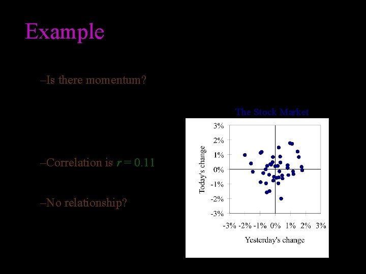
Example –Is there momentum? • If the market was up yesterday, is it more likely to be up today? • Or is each day’s performance independent? –Correlation is r = 0. 11 • A weak relationship? –No relationship? • Tilt is neither up nor down The Stock Market

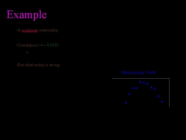
Example –A nonlinear relationship • Not a straight line: A curved relationship –Correlation r = – 0. 0155 • r suggests no relationship but in reality there is a relationship it is just NOT linear –But relationship is strong Maximizing Yield of process • It tilts neither up nor down 160 150 140 130 120 500 600 700 800 Temperature 900

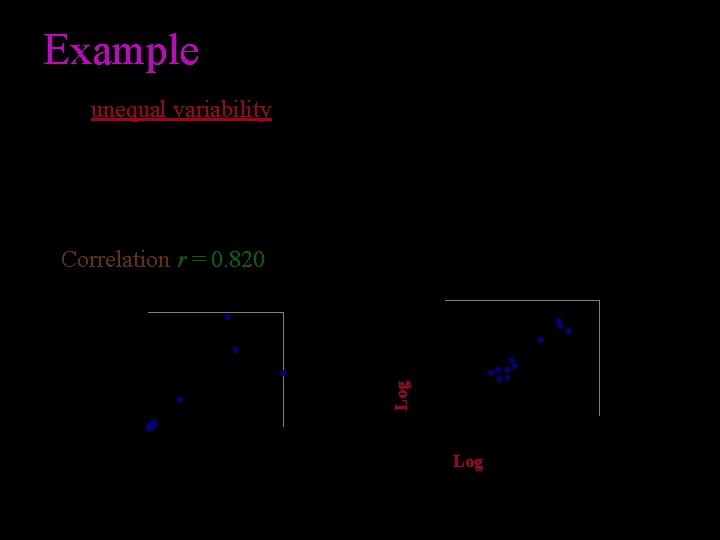
Example unequal variability Variability is stabilized by taking logarithms (lower right Correlation r = 0. 820 investment Log of miles Circuit miles (millions) investment 2, 000 1, 000 0 0 1, 000 2, 000 Investment ($millions) 20 15 15 20 Log of investment

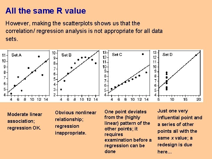
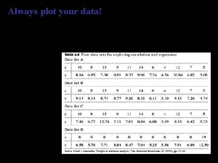
All the same R value However, making the scatterplots shows us that the correlation/ regression analysis is not appropriate for all data sets. Moderate linear association; regression OK. Obvious nonlinear relationship; regression inappropriate. One point deviates from the (highly linear) pattern of the other points; it requires examination before a regression can be done Just one very influential point and a series of other points all with the same x value; a redesign is due here…

Always plot your data! The correlations all give r ≈ 0. 816, and the regression lines are all approximately = 3 + 0. 5 x. For all four sets, we would predict = 8 when x = 10. The previous slides data.

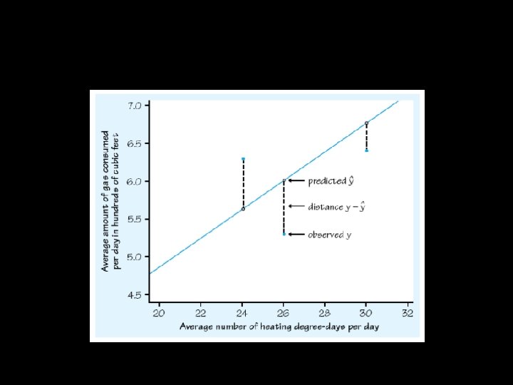
We want the line as close as possible to the points.

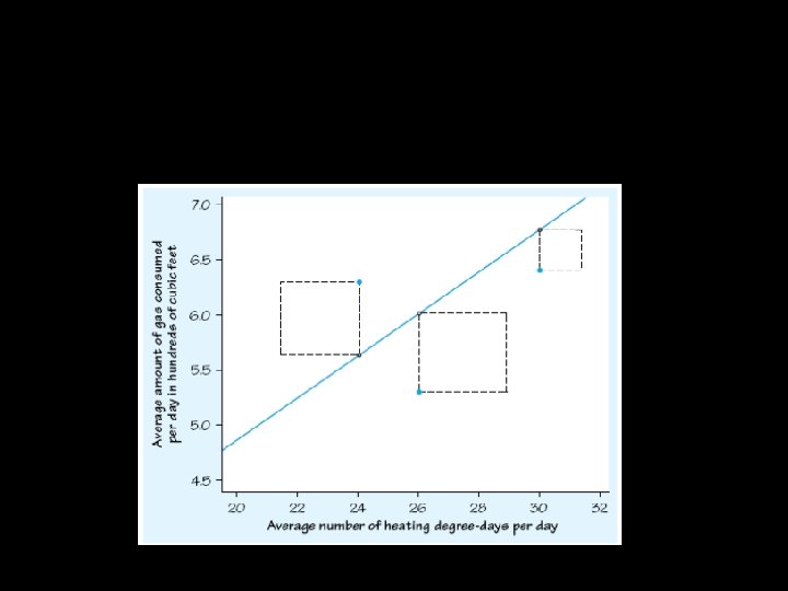
So, we need the line that will minimize the sum of the squares of the vertical distances.

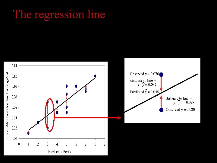
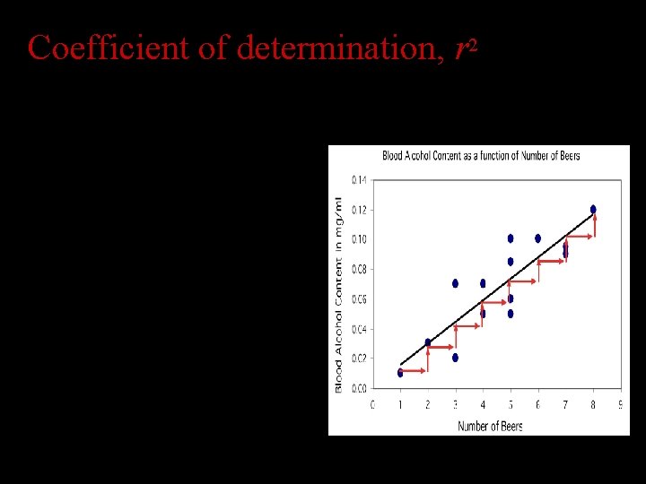
The regression line The least-squares regression line is the unique line such that the sum of the squared vertical (y) distances between the data points and the line is the smallest possible. BAC levels Distances between the points and line are squared so all are positive values. This is done so that distances can be properly added

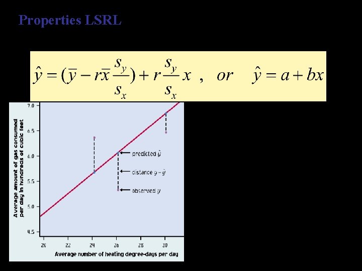
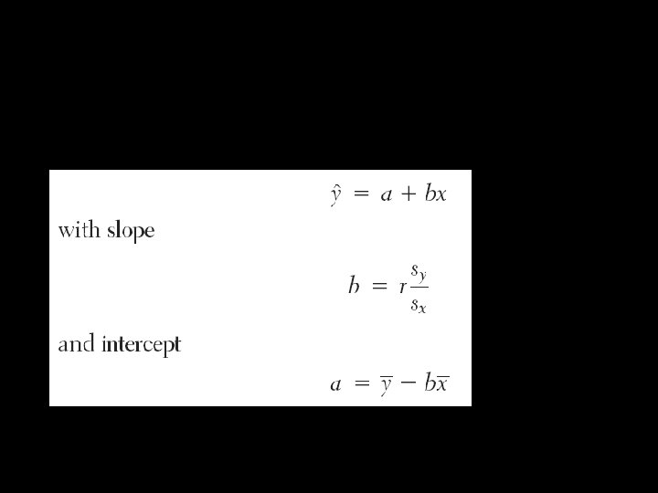
Properties LSRL The least-squares regression line can be shown to have this equation: is the predicted y value (y hat) b is the slope a is the y-intercept "a" is in units of y "b" is in units of y/units of x

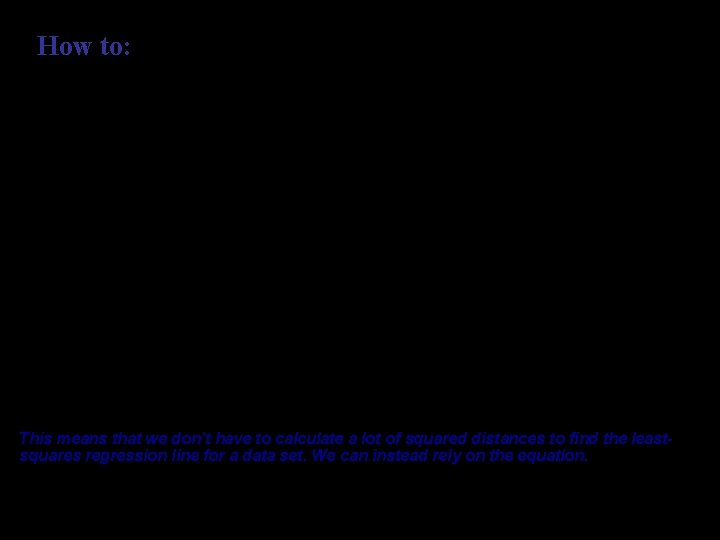
How to: First we calculate the slope of the line, b, from statistics we already know: r is the correlation sy is the standard deviation of the response variable y sx is the standard deviation of the explanatory variable x Once we know b, the slope, we can calculate a, the y-intercept: where x and y are the sample means of the x and y variables This means that we don’t have to calculate a lot of squared distances to find the leastsquares regression line for a data set. We can instead rely on the equation.

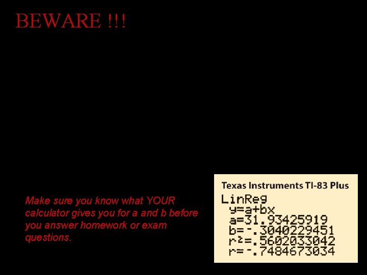
BEWARE !!! Not all calculators and software use the same convention: We use this one: Ti-89 and Ti-83 give both Some use instead: Make sure you know what YOUR calculator gives you for a and b before you answer homework or exam questions.

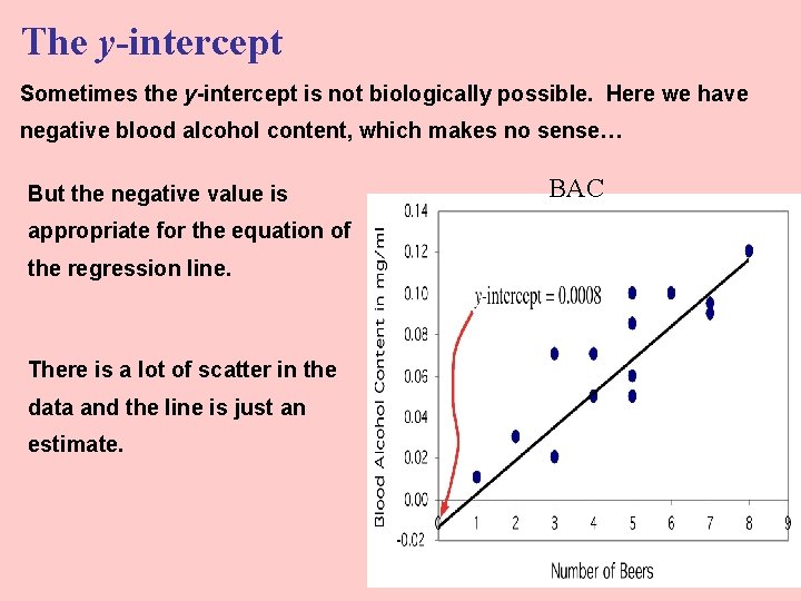
The y-intercept Sometimes the y-intercept is not biologically possible. Here we have negative blood alcohol content, which makes no sense… But the negative value is appropriate for the equation of the regression line. There is a lot of scatter in the data and the line is just an estimate. BAC

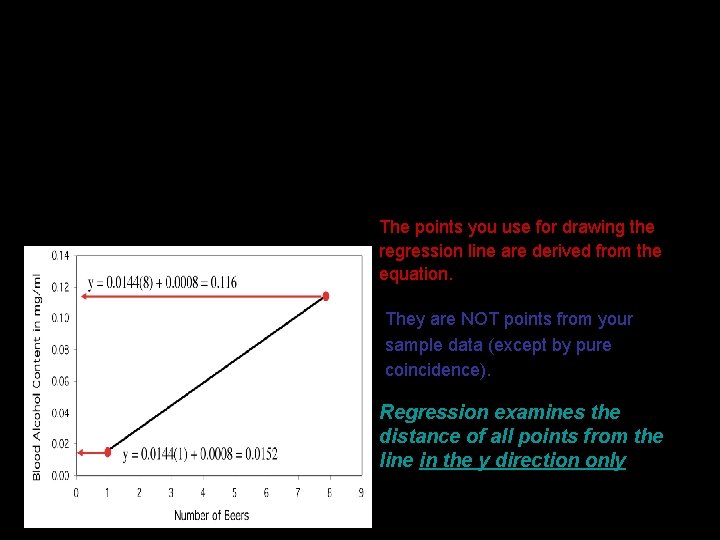
The equation completely describes the regression line. To plot the regression line, you only need to plug two x values into the equation, get y, and draw the line that goes through those two points. Hint: The regression line always passes through the mean of x and y Thus: The points you use for drawing the regression line are derived from the equation. They are NOT points from your sample data (except by pure coincidence). Regression examines the distance of all points from the line in the y direction only

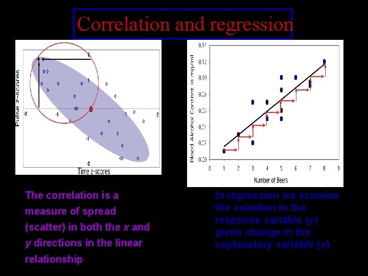
Correlation and regression The correlation is a measure of spread (scatter) in both the x and y directions in the linear relationship In regression we examine the variation in the response variable (y) given change in the explanatory variable (x)

Equations The general form for a regression line is

Coefficient of determination, r 2 • It measures the fraction (or percent) of the variation in y that is explained by the least squares regression line of y on x. (Memorize this sentence!) • Basically, this helps us interpret r in a more understandable way since r 2 is a percent.

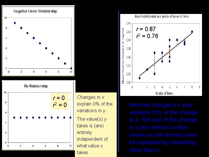
Coefficient of determination, r 2, the coefficient of determination, is the square of the correlation coefficient r r 2 represents the percentage of the variance in y (vertical scatter from the regression line) that can be explained by changes in x.

Changes in x explain 100% of the variations in y. r = 0. 87 r 2 = 0. 76 y can be entirely predicted for any given value of x. r=0 r 2 = 0 Changes in x explain 0% of the variations in y. The value(s) y takes is (are) entirely independent of what value x takes. Here the change in x only explains 76% of the change in y. The rest of the change in y (the vertical scatter, shown as red arrows) must be explained by something other than x.

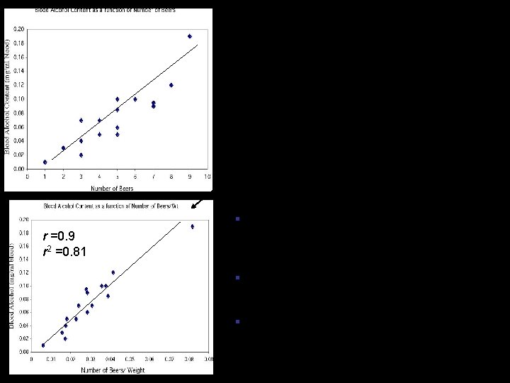
There is quite some variation in BAC for the same number of beers drunk. A person’s blood volume is a factor in the equation that was overlooked here. We changed the number of beers to the number of beers/weight of a person in pounds. r =0. 9 r 2 =0. 81 §In the first plot, number of beers only explains 49% of the variation in blood alcohol content. §But number of beers/weight explains 81% of the variation in blood alcohol content. §Additional factors contribute to variations in BAC among individuals (like maybe some genetic ability to process alcohol).

Grade performance If class attendance explains 16% of the variation in grades, what is the correlation between percent of classes attended and grade? 1. We need to make an assumption: Attendance and grades are positively correlated. So r will be positive too. 2. r 2 = 0. 16, so r = +√ 0. 16 = + 0. 4 A weak correlation.

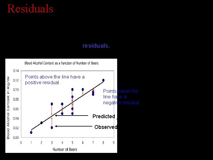
Residuals The distances from each point to the least-squares regression line give us potentially useful information about the contribution of individual data points to the overall pattern of scatter. These distances are called “residuals. ” The sum of these residuals is always 0 Points above the line have a positive residual. Points below the line have a negative residual Predicted y^ Observed y

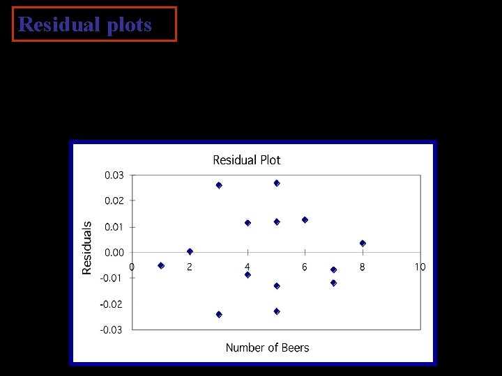
Residual plots Residuals are the distances between y-observed and y-predicted. We plot them in a residual plot. If residuals are scattered randomly around 0, chances are your data fit a linear model, were normally distributed, and you didn’t have outliers

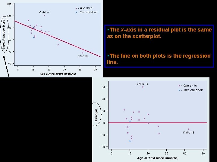
§The x-axis in a residual plot is the same as on the scatterplot. §The line on both plots is the regression line. Only the y-axis is different

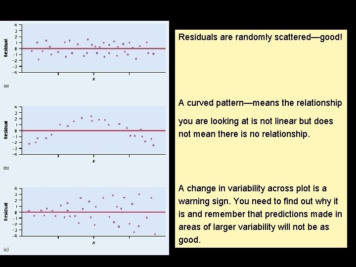
Residuals are randomly scattered—good! A curved pattern—means the relationship you are looking at is not linear but does not mean there is no relationship. A change in variability across plot is a warning sign. You need to find out why it is and remember that predictions made in areas of larger variability will not be as good.

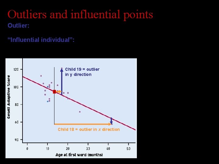
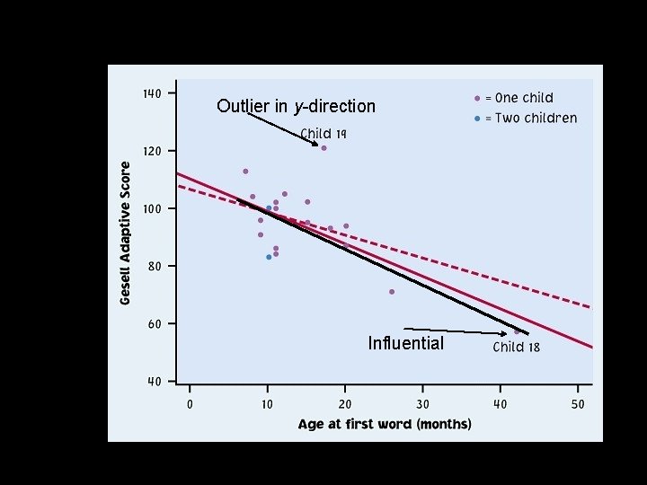
Outliers and influential points Outlier: An observation that lies outside the overall pattern of observations. “Influential individual”: An observation that markedly changes the regression if removed. This is often an outlier on the x-axis. Child 19 = outlier in y direction Child 19 is an outlier of the relationship. Child 18 = outlier in x direction Child 18 is only an outlier in the x direction and thus might be an influential point.

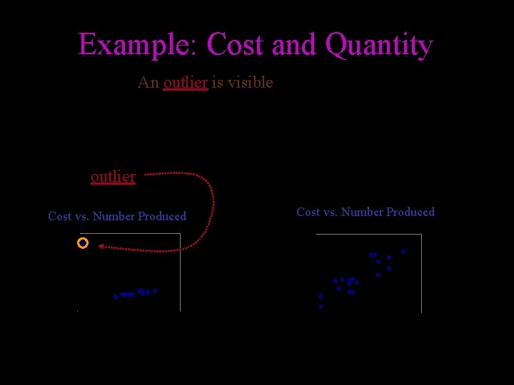
Example: Cost and Quantity An outlier is visible • A disaster (a fire at the factory) • High cost, but few produced outlier Outlier removed Cost vs. Number Produced Cost 5, 000 10, 000 4, 000 0 0 20 40 60 Number produced 3, 000 20 30 40 50 Number produced

Outlier in y-direction Are these points influential? Influential

OUTLIERS IN TERMS OF REGRESSION: Observations with large (in absolute value) residuals. Observations falling f a r from the regression line while not following the pattern of the relationship apparent in the others Residual=actual-fitted Residual = y-y(hat)

INFLUENTIAL POINTS ARE: Points whose removal would greatly affect the association of two variables Points whose removal would significantly change the slope of an LSR line Points with a large moment (i. e they are far away from the rest of the data. ) Usually outliers in the x direction.

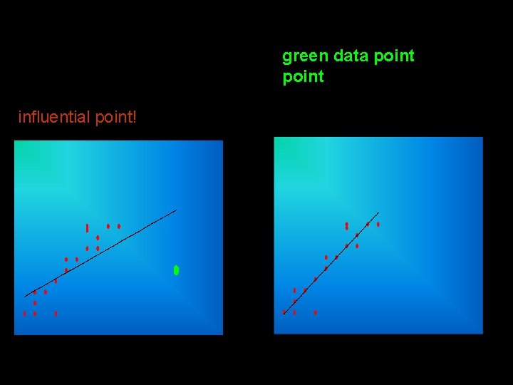
The two graphs below show the same data – the on the right with the removal of the green data point. As you can see, the removal of this point significantly affects the slope of the regression line. This is an influential point!

!!!REMEMBER!!! An observation does NOT have to be an Outlier to be an Influential Point!! Nor does an observation need to be an Influential Point in order to be an Outlier!!

Given the five-number summary {8 21 35 43 77}, which of the following is correct? A. There are no outliers B. There at least two outliers C. There is not enough data to make any conclusion D. There is exactly one outlier E. There is at least one outlier

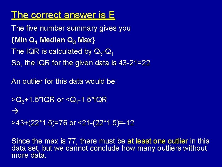
The correct answer is E The five number summary gives you {Min Q 1 Median Q 3 Max} The IQR is calculated by Q 3 -Q 1 So, the IQR for the given data is 43 -21=22 An outlier for this data would be: >Q 3+1. 5*IQR or <Q 1 -1. 5*IQR >43+(22*1. 5)=76 or <21 -(22*1. 5)=-12 Since the max is 77, there must be at least one outlier in this data set, but we cannot conclude how many outliers without more data.

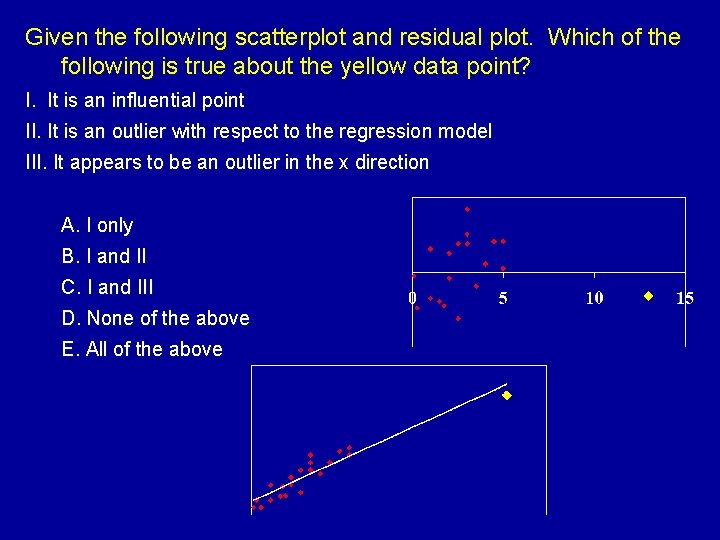
Given the following scatterplot and residual plot. Which of the following is true about the yellow data point? I. It is an influential point II. It is an outlier with respect to the regression model III. It appears to be an outlier in the x direction A. I only B. I and II C. I and III D. None of the above E. All of the above

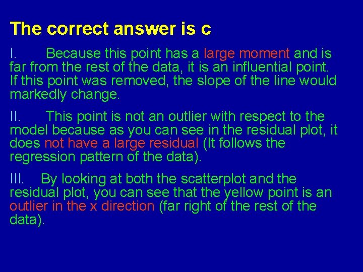
The correct answer is c I. Because this point has a large moment and is far from the rest of the data, it is an influential point. If this point was removed, the slope of the line would markedly change. II. This point is not an outlier with respect to the model because as you can see in the residual plot, it does not have a large residual (It follows the regression pattern of the data). III. By looking at both the scatterplot and the residual plot, you can see that the yellow point is an outlier in the x direction (far right of the rest of the data).

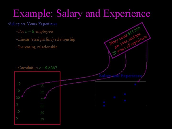
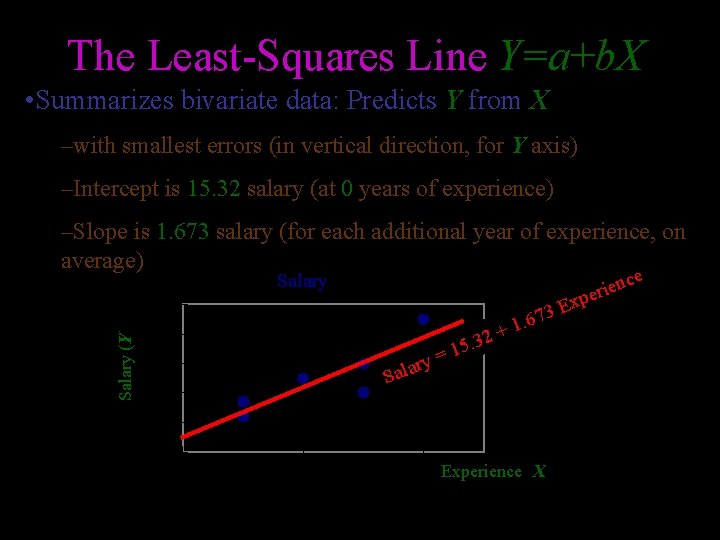
Example: Salary and Experience • Salary vs. Years Experience 000 , 5 $5 has s n ar and ience e ry ear, per a M r y f ex pe rs o yea 0 2 –For n = 6 employees –Linear (straight line) relationship –Increasing relationship • higher salary generally goes with higher experience –Correlation r = 0. 8667 Salary 15 30 10 35 20 55 5 22 15 40 5 27 Salary and Experience Salary ($thousand) Experience 60 50 40 30 20 0 10 20 Experience

The Least-Squares Line Y=a+b. X • Summarizes bivariate data: Predicts Y from X –with smallest errors (in vertical direction, for Y axis) –Intercept is 15. 32 salary (at 0 years of experience) –Slope is 1. 673 salary (for each additional year of experience, on average) e nc e i r pe Salary x Salary (Y) 60 50 ry a l a S 40 30 = 2 15. 3 + E 3 7 6 1. 20 10 20 Experience (X)

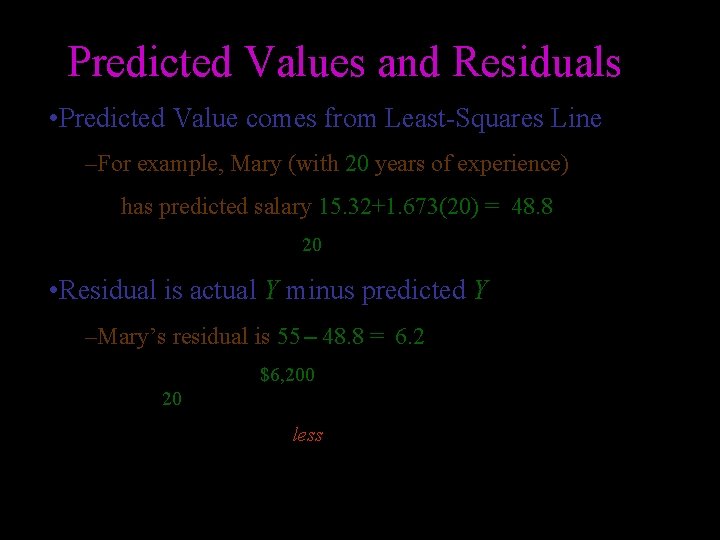
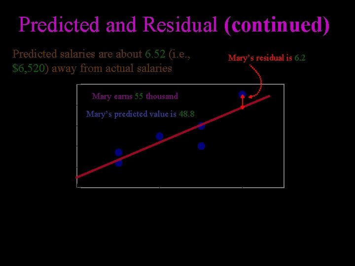
Predicted Values and Residuals • Predicted Value comes from Least-Squares Line –For example, Mary (with 20 years of experience) has predicted salary 15. 32+1. 673(20) = 48. 8 • So does anyone with 20 years of experience • Residual is actual Y minus predicted Y –Mary’s residual is 55 – 48. 8 = 6. 2 • She earns about $6, 200 more than the predicted salary for a person with 20 years of experience • A person who earns less than predicted will have a negative residual

Predicted and Residual (continued) Predicted salaries are about 6. 52 (i. e. , $6, 520) away from actual salaries Mary’s residual is 6. 2 60 Mary earns 55 thousand 50 Mary’s predicted value is 48. 8 Salary 40 30 20 10 Experience 20

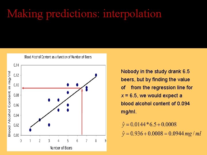
Making predictions: interpolation The equation of the least-squares regression allows you to predict y for any x within the range studied. This is called interpolating. Nobody in the study drank 6. 5 beers, but by finding the value of from the regression line for x = 6. 5, we would expect a blood alcohol content of 0. 094 mg/ml.

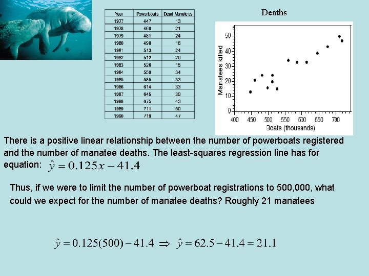
Deaths There is a positive linear relationship between the number of powerboats registered and the number of manatee deaths. The least-squares regression line has for equation: Thus, if we were to limit the number of powerboat registrations to 500, 000, what could we expect for the number of manatee deaths? Roughly 21 manatees

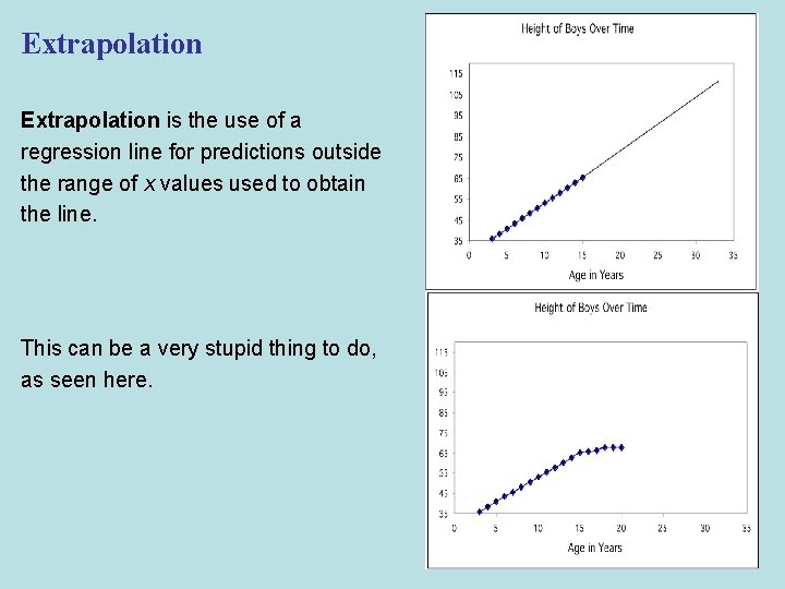
Extrapolation is the use of a regression line for predictions outside the range of x values used to obtain the line. This can be a very stupid thing to do, as seen here.

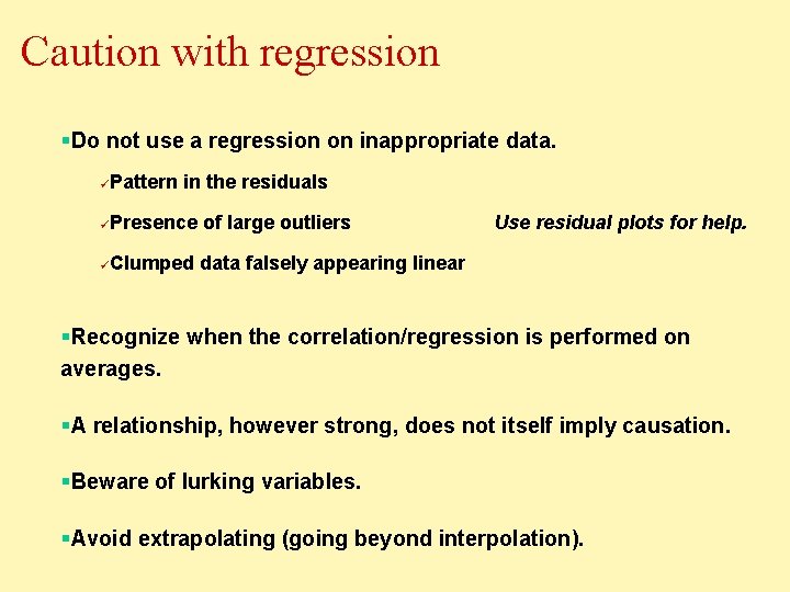
Caution with regression §Do not use a regression on inappropriate data. üPattern in the residuals üPresence of large outliers üClumped data falsely appearing linear Use residual plots for help. §Recognize when the correlation/regression is performed on averages. §A relationship, however strong, does not itself imply causation. §Beware of lurking variables. §Avoid extrapolating (going beyond interpolation).