AP Macro PHILLIPS CURVE LAFFER CURVE The Phillips

AP Macro PHILLIPS CURVE LAFFER CURVE

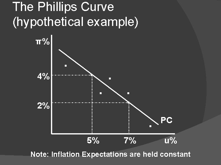
The Phillips Curve � In a 1958 paper, New Zealand born economist, A. W. Phillips published the results of his research on the historical relationship between the unemployment rate (u%) and the rate of inflation (π%) in Great Britain. His research indicated a stable inverse relationship between the u% and the π%. As u%↓, π%↑ ; and as u%↑, π%↓. The implication of this relationship was that policy makers could exploit the trade-off and reduce u% at the cost of increased π%. The Phillips curve was used as a rationale for the Keynesian aggregate demand policies of the mid-20 th century.

A. W. Phillips � It’s customary in a presentation to include the picture of the person whose work is being studied. I didn’t have much luck, but here’s what I’ve got. I like to think that Phillips looked like this. Thanks Google.

The Phillips Curve (hypothetical example) π% 4% 2% . . . 5% 7% . PC u% Note: Inflation Expectations are held constant

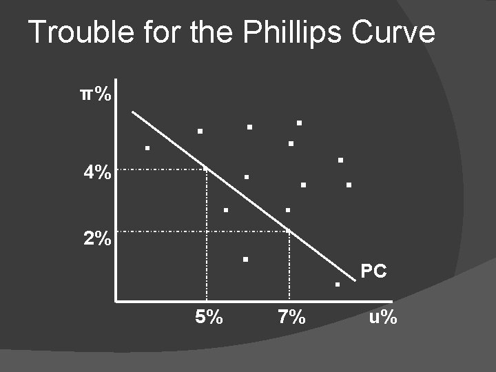
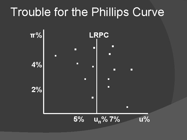
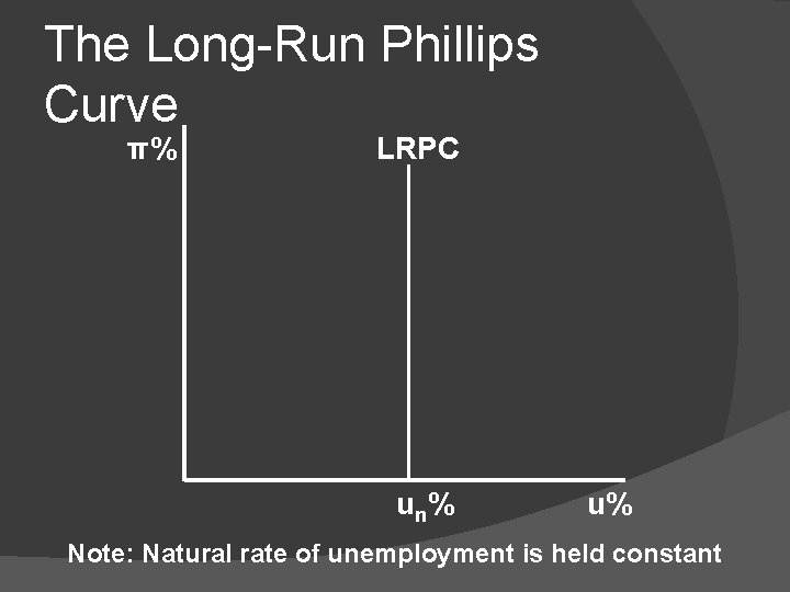
Trouble for the Phillips Curve � In the 1970’s the United States experienced concurrent high u% & π%, a condition known as stagflation. 1976 American Nobel Prize economist Milton Friedman saw stagflation as disproof of the stable Phillips Curve. Instead of a trade-off between u% & π%, Friedman and 2006 Nobel Prize recipient Edmund Phelps believed that the natural u% was independent of the π%. This independent relationship is now referred to as the Long-Run Phillips Curve. I believe it’s relevant that by this time the Bretton. Woods system had collapsed.

Trouble for the Phillips Curve π% 4% 2% . . . 5% 7% . PC u%

Trouble for the Phillips Curve π% 4% 2% LRPC . . . 5% un% 7% . u%

The Long-Run Phillips Curve π% LRPC u n% u% Note: Natural rate of unemployment is held constant

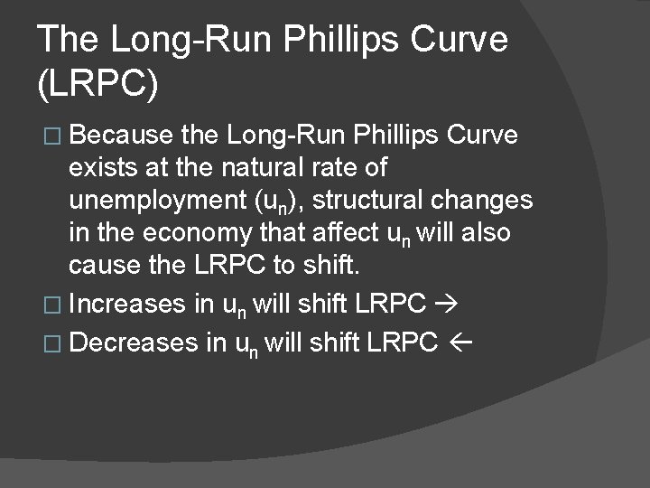
The Long-Run Phillips Curve (LRPC) � Because the Long-Run Phillips Curve exists at the natural rate of unemployment (un), structural changes in the economy that affect un will also cause the LRPC to shift. � Increases in un will shift LRPC � Decreases in un will shift LRPC

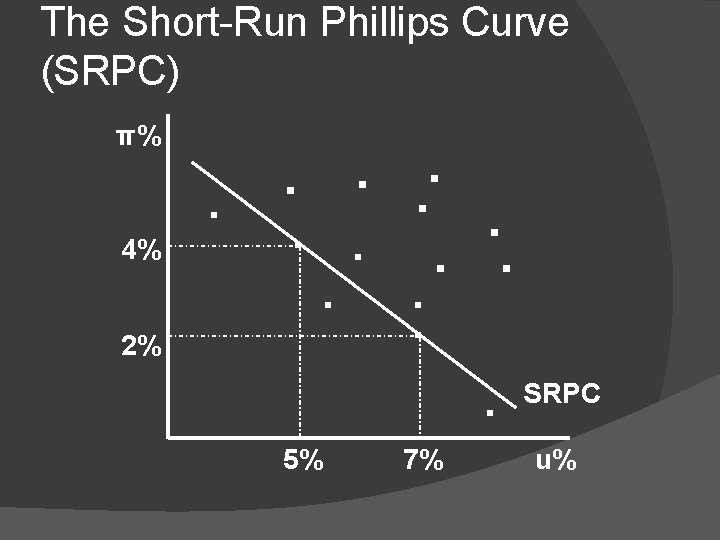
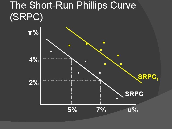
The Short-Run Phillips Curve (SRPC) � Today many economists reject the concept of a stable Phillips curve, but accept that there may be a short-term trade-off between u% & π% given stable inflation expectations. Most believe that in the long-run u% & π% are independent at the natural rate of unemployment. Modern analysis shows that the SRPC may shift left or right. The key to understanding shifts in the Phillips curve is inflationary expectations!

The Short-Run Phillips Curve (SRPC) π% 4% 2% . . . 5% 7% . SRPC u%

The Short-Run Phillips Curve (SRPC) π% 4% 2% . . . 5% 7% SRPC 1 . SRPC u%

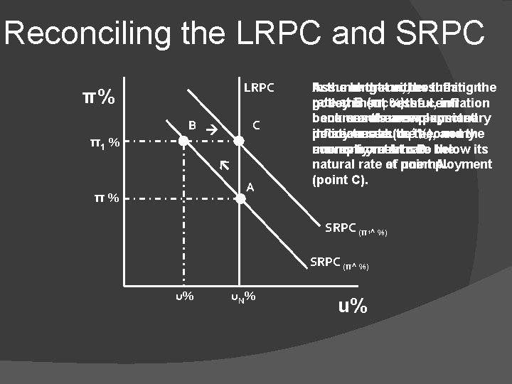
Reconciling the LRPC and SRPC LRPC π% C π1 % B A π% Assume long-run, that either the inflationthe In the short-run, assuming rate at is B successful, (π1 or %) the central government policy inflation becomes bank enacts the an new expansionary expected occurs and unemployment ^%), inflation policy to rate reduce and the decreases as(π the economy 1 the economy unemployment returns rate to below the its moves from A to B. natural rate at of point unemployment A. (point C). SRPC (π1^ %) SRPC (π^ %) u% u. N% u%

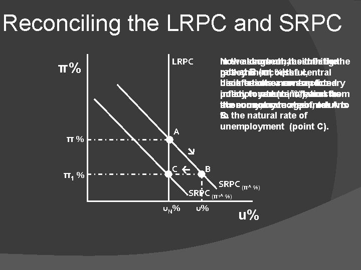
Reconciling the LRPC and SRPC π% π% LRPC In theassume long-run, short-run, the assuming inflation Now that either thethe rate at is B successful, (π1 or %) the central policy government becomes disinflation the occurs expected and bank enacts anew contractionary ^inflation unemployment (π1 increases %), and the as policy to rate reduce from economy, the economy once moves again, from returns it’s current rate at point A A to to the natural rate of B. unemployment (point C). A C π1 % B SRPC (π^ %) SRPC (π1^ %) u. N% u% u%

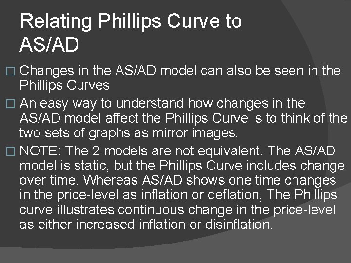
Relating Phillips Curve to AS/AD Changes in the AS/AD model can also be seen in the Phillips Curves � An easy way to understand how changes in the AS/AD model affect the Phillips Curve is to think of the two sets of graphs as mirror images. � NOTE: The 2 models are not equivalent. The AS/AD model is static, but the Phillips Curve includes change over time. Whereas AS/AD shows one time changes in the price-level as inflation or deflation, The Phillips curve illustrates continuous change in the price-level as either increased inflation or disinflation. �

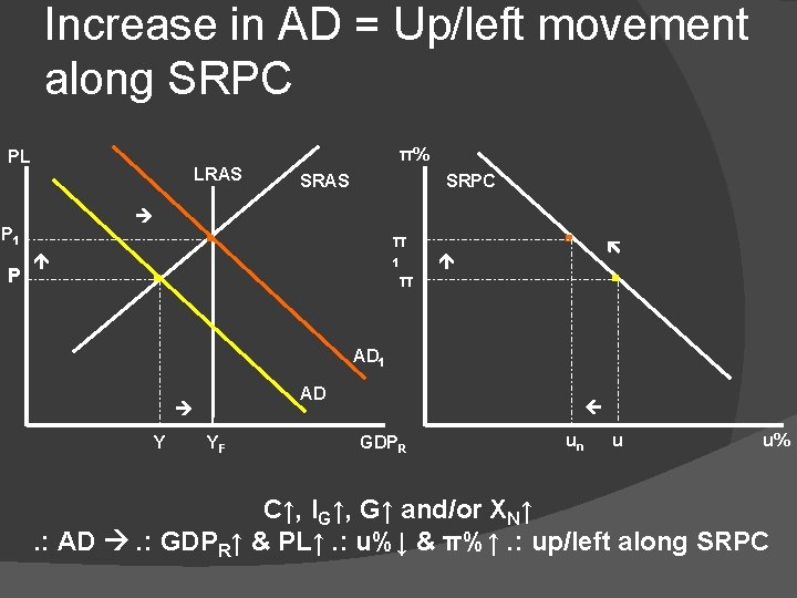
Increase in AD = Up/left movement along SRPC π% PL LRAS SRPC 1 π . . π P 1 AD Y YF P . . SRAS GDPR un u u% C↑, IG↑, G↑ and/or XN↑. : AD . : GDPR↑ & PL↑. : u%↓ & π%↑. : up/left along SRPC

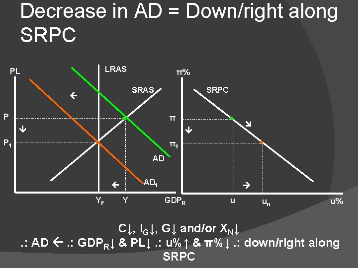
Decrease in AD = Down/right along SRPC LRAS PL . SRPC π . π1 . AD AD 1 P 1 SRAS . P π% YF Y GDPR u un u% C↓, IG↓, G↓ and/or XN↓. : AD . : GDPR↓ & PL↓. : u%↑ & π%↓. : down/right along SRPC

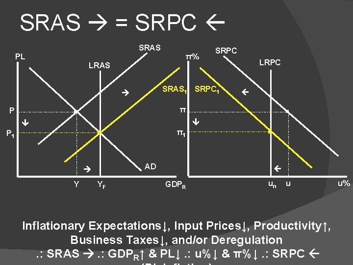
SRAS = SRPC SRAS PL π% SRPC LRAS . . GDPR un AD Y π1 YF . P 1 π . P SRAS 1 SRPC 1 u Inflationary Expectations↓, Input Prices↓, Productivity↑, Business Taxes↓, and/or Deregulation. : SRAS . : GDPR↑ & PL↓. : u%↓ & π%↓. : SRPC u%

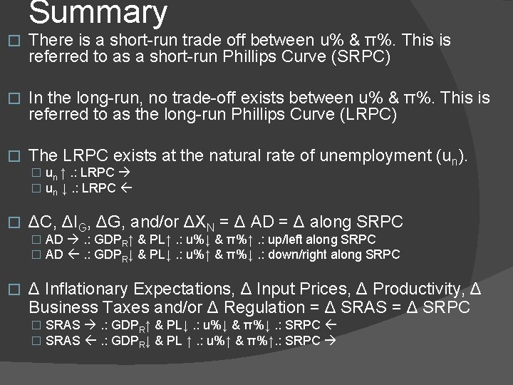
Summary � There is a short-run trade off between u% & π%. This is referred to as a short-run Phillips Curve (SRPC) � In the long-run, no trade-off exists between u% & π%. This is referred to as the long-run Phillips Curve (LRPC) � The LRPC exists at the natural rate of unemployment (un). � un ↑. : LRPC � un ↓. : LRPC � ΔC, ΔIG, ΔG, and/or ΔXN = Δ AD = Δ along SRPC � AD . : GDPR↑ & PL↑. : u%↓ & π%↑. : up/left along SRPC � AD . : GDPR↓ & PL↓. : u%↑ & π%↓. : down/right along SRPC � Δ Inflationary Expectations, Δ Input Prices, Δ Productivity, Δ Business Taxes and/or Δ Regulation = Δ SRAS = Δ SRPC � SRAS . : GDPR↑ & PL↓. : u%↓ & π%↓. : SRPC � SRAS . : GDPR↓ & PL ↑. : u%↑ & π%↑. : SRPC

Arthur Laffers Curve

The Laffer Curve � Arthur Laffer is a supply side economist who became influential during the Reagan administration as a member of Reagan's Economic Policy Advisory Board (1981 -1989).

Supply Side Economics Based idea � Reductions in marginal tax rates increase the nation’s aggregate supply. � The Laffer Curve depicts the relationship between tax rates and tax revenues.

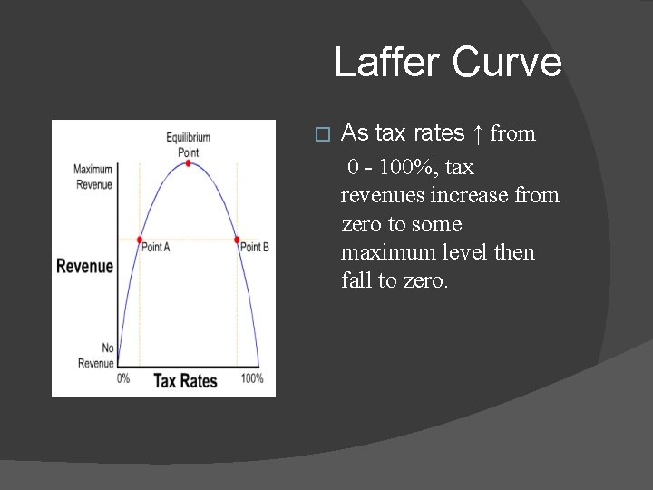
Laffer Curve � As tax rates ↑ from 0 - 100%, tax revenues increase from zero to some maximum level then fall to zero.

Laffer Curve Tax revenues decline beyond some point because higher tax rates discourage economic activity, therefore shrinking the tax base. � When taxes are lower, tax avoidance and tax evasion is less. � If tax rate is 100%, revenue is reduced to zero because a 100% rate has halted production. � A 100% tax rate=0 revenue �

Criticisms of the Laffer The degree economic incentives are sensitive to changes in the tax rate. ↓ taxes encourages others to work more, while some work less. ↓after tax pay encourages ↑work, ↑ after tax pay encourages ↓work. 2. Inflation-demand side effects of a tax cut exceed the supply-side effects. Demand pull inflation is likely. 3. Position on the curve-an economies position on the curve is undocumented and unknown. 1.