AOSS 401 Geophysical Fluid Dynamics Atmospheric Dynamics Prepared

AOSS 401 Geophysical Fluid Dynamics: Atmospheric Dynamics Prepared: 20131119 Quasi-geostrophic / Waves / Vertical / Richard B. Rood (Room 2525, SRB) rbrood@umich. edu 734 -647 -3530 Cell: 301 -526 -8572

Class News • Ctools site (AOSS 401 001 F 13) • Second Examination on December 10, 2013 • Homework – Posted Today

Weather • National Weather Service – Model forecasts: • Weather Underground – Model forecasts: • NCAR Research Applications Program

Outline • • Waves In Class Problem Quasi-geostrophic Review Vertical Velocity

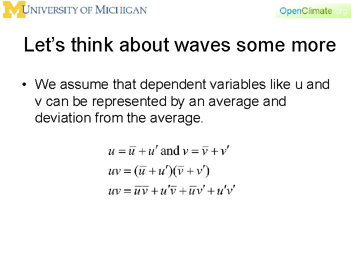
Let’s think about waves some more • We assume that dependent variables like u and v can be represented by an average and deviation from the average.

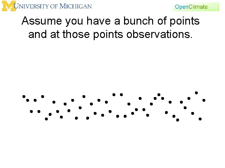
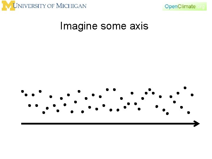
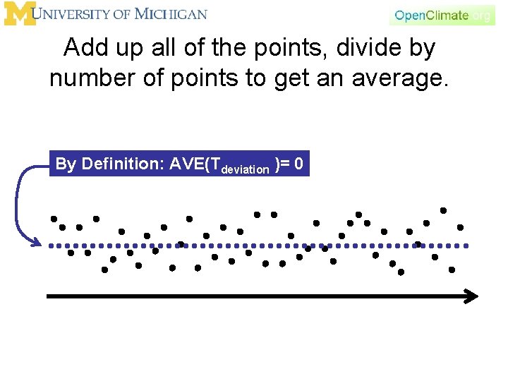
Assume you have a bunch of points and at those points observations.

Imagine some axis

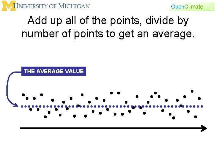
Add up all of the points, divide by number of points to get an average. THE AVERAGE VALUE

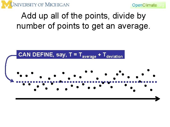
Add up all of the points, divide by number of points to get an average. CAN DEFINE, say, T = Taverage + Tdeviation

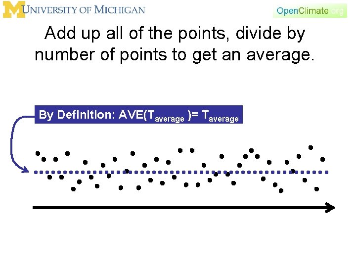
Add up all of the points, divide by number of points to get an average. By Definition: AVE(Taverage )= Taverage

Add up all of the points, divide by number of points to get an average. By Definition: AVE(Tdeviation )= 0

The averaging • We can define spatial averages or we can define time averages.

The averaging • We can define spatial averages or we can define time averages. • When we define a spatial average, say over the east-west direction, x, all the way around the globe, the average is NOT a function of variable over which we averaged. ∂ave(T)/∂x=0

The averaging • We can define spatial averages or we can define time averages. • When we define a time average, especially when we are developing theory, we can say that the average changes slowly with time, while the perturbation changes rapidly in time. ∂ave(T)/∂t not required to be 0 But the perturbations still average to zero, because we assume that the average is over a long span of time compared with the perturbation time scale. THINK ABOUT IT. . . Define, use the definitions.

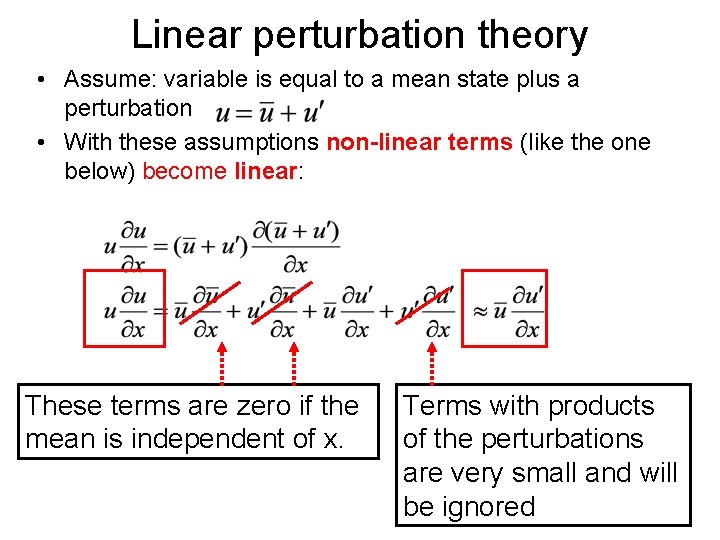
Linear perturbation theory • Assume: variable is equal to a mean state plus a perturbation • With these assumptions non-linear terms (like the one below) become linear: These terms are zero if the mean is independent of x. Terms with products of the perturbations are very small and will be ignored

Waves • The equations of motion contain many forms of wave-like solutions, true for the atmosphere and ocean • Some are of interest depending on the problem: Rossby waves, internal gravity (buoyancy) waves, inertial-gravity waves, topographic waves, shallow water gravity waves • Some are not of interest to meteorologists, e. g. sound waves • Waves transport energy, mix the air (especially when breaking)

Waves • Large-scale mid-latitude waves, are critical for weather forecasting and transport. • Large-scale waves in the tropics (Kelvin waves, mixed Rossby-gravity waves) are also important, but of very different character. Will introduce these after the next test; this is focus of AOSS 451. • This is true for both ocean and atmosphere. • Waves can be unstable. That is they start to grow, rather than just bounce back and forth.

Outline • • Waves In Class Problem Quasi-geostrophic Review Vertical Velocity

In class problems • Group (Thermal) – Scott – Anna – James – Kevin – Trent • Group (Perturb) – John – Ross – Rachel – Jordan – Justin – Alex

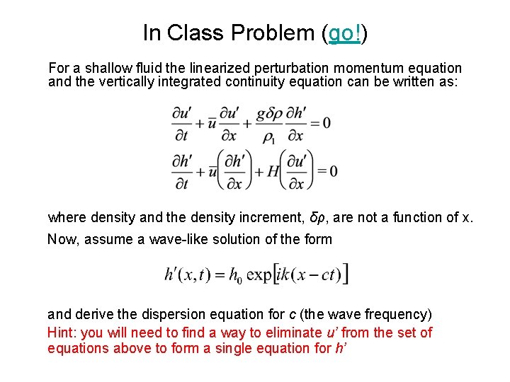
In Class Problem (go!) For a shallow fluid the linearized perturbation momentum equation and the vertically integrated continuity equation can be written as: where density and the density increment, δρ, are not a function of x. Now, assume a wave-like solution of the form and derive the dispersion equation for c (the wave frequency) Hint: you will need to find a way to eliminate u’ from the set of equations above to form a single equation for h’

Outline • • Waves In Class Problem Quasi-geostrophic Review Vertical Velocity

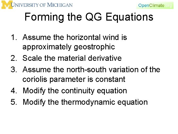
Forming the QG Equations 1. Assume the horizontal wind is approximately geostrophic 2. Scale the material derivative 3. Assume the north-south variation of the coriolis parameter is constant 4. Modify the continuity equation 5. Modify thermodynamic equation

Scaled equations of motion in pressure coordinates Definition of geostrophic wind Momentum equation Continuity equation Thermodynamic Energy equation

Remember the relationship between vorticity and geopotential

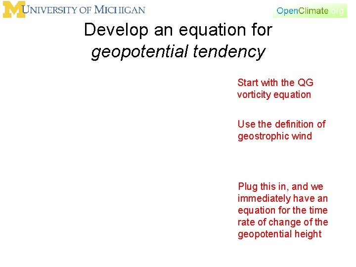
Develop an equation for geopotential tendency Start with the QG vorticity equation Use the definition of geostrophic wind Plug this in, and we immediately have an equation for the time rate of change of the geopotential height

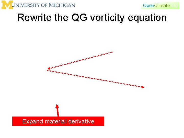
Rewrite the QG vorticity equation Expand material derivative

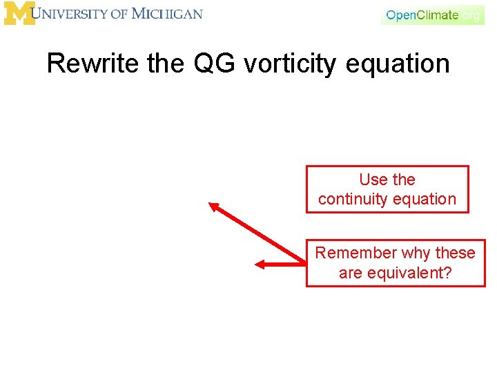
Rewrite the QG vorticity equation Use the continuity equation Remember why these are equivalent?

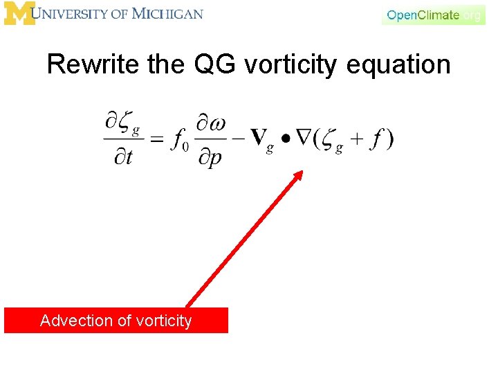
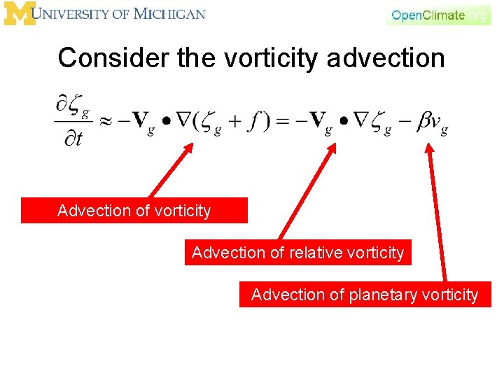
Rewrite the QG vorticity equation Advection of vorticity

Consider the vorticity advection Advection of vorticity Advection of relative vorticity Advection of planetary vorticity

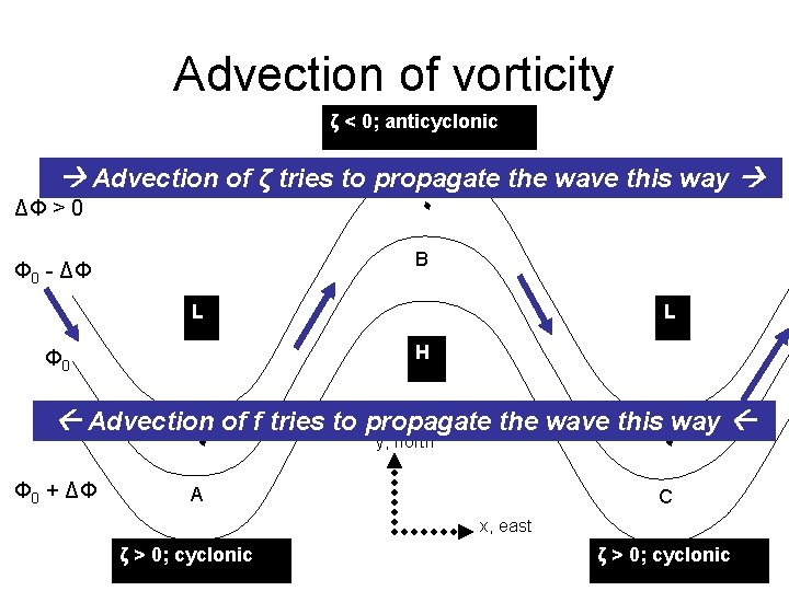
Summary: Vorticity Advection in Wave • Planetary and relative vorticity advection in a wave oppose each other. • This is consistent with our observation of trade-off between relative and planetary vorticity in westerly flow over a mountain range

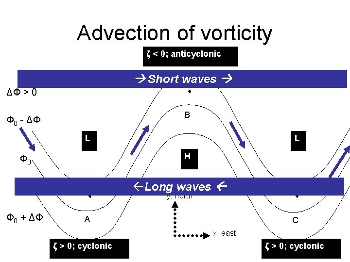
Advection of vorticity ζ < 0; anticyclonic Advection of ζ tries to propagate the wave this way ٠ ΔΦ > 0 B Φ 0 - ΔΦ L L H Φ 0 Advection of f tries to propagate the wave this way ٠ Φ 0 + ΔΦ ٠ y, north A C x, east ζ > 0; cyclonic

Idealized solution: Barotropic Vorticity

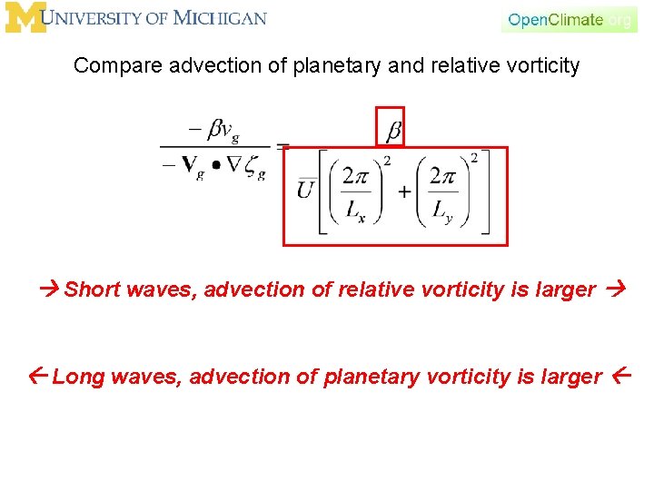
Compare advection of planetary and relative vorticity Short waves, advection of relative vorticity is larger Long waves, advection of planetary vorticity is larger

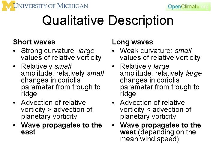
Qualitative Description Short waves • Strong curvature: large values of relative vorticity • Relatively small amplitude: relatively small changes in coriolis parameter from trough to ridge • Advection of relative vorticity > advection of planetary vorticity • Wave propagates to the east Long waves • Weak curvature: small values of relative vorticity • Relatively large amplitude: relatively large changes in coriolis parameter from trough to ridge • Advection of relative vorticity < advection of planetary vorticity • Wave propagates to the west (depending on the mean wind speed)

Advection of vorticity ζ < 0; anticyclonic Short waves ٠ ΔΦ > 0 B Φ 0 - ΔΦ L H Φ 0 ٠ Φ 0 + ΔΦ L ßLong waves y, north A ٠ C x, east ζ > 0; cyclonic

A more general equation for geopotential tendency

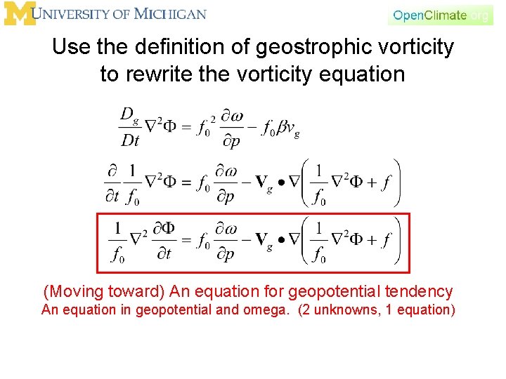
Use the definition of geostrophic vorticity to rewrite the vorticity equation (Moving toward) An equation for geopotential tendency An equation in geopotential and omega. (2 unknowns, 1 equation)

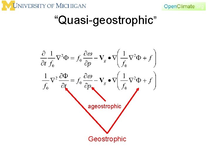
“Quasi-geostrophic” ageostrophic Geostrophic

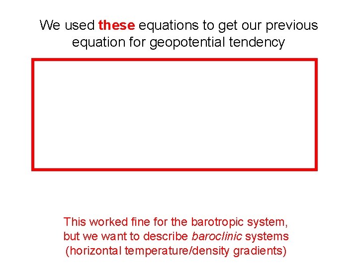
We used these equations to get our previous equation for geopotential tendency This worked fine for the barotropic system, but we want to describe baroclinic systems (horizontal temperature/density gradients)

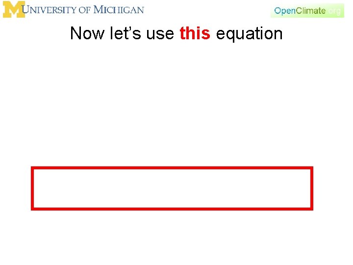
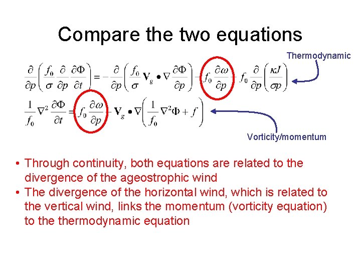
Now let’s use this equation

Compare the two equations Thermodynamic Vorticity/momentum • Through continuity, both equations are related to the divergence of the ageostrophic wind • The divergence of the horizontal wind, which is related to the vertical wind, links the momentum (vorticity equation) to thermodynamic equation

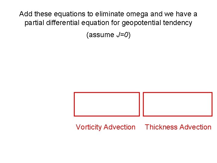
Add these equations to eliminate omega and we have a partial differential equation for geopotential tendency (assume J=0) Vorticity Advection Thickness Advection

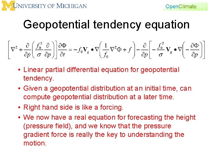
Geopotential tendency equation • Linear partial differential equation for geopotential tendency. • Given a geopotential distribution at an initial time, can compute geopotential distribution at a later time. • Right hand side is like a forcing. • We now have a real equation forecasting the height (pressure field), and we know that the pressure gradient force is really the key to understanding the motion.

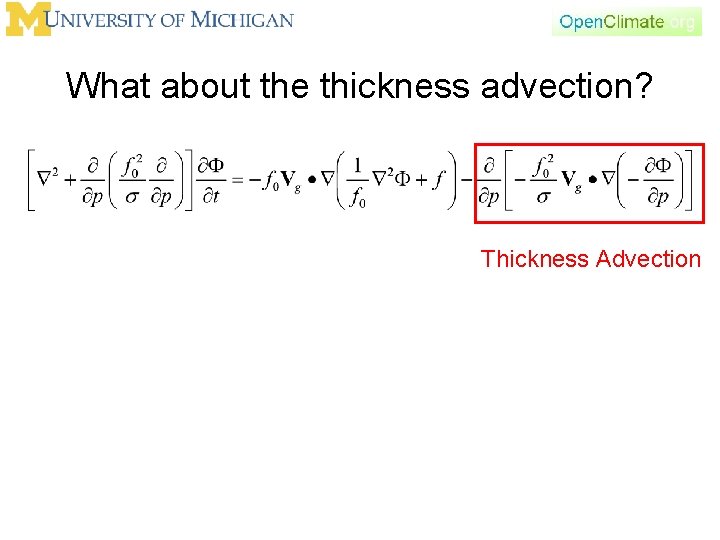
What about the thickness advection? Thickness Advection

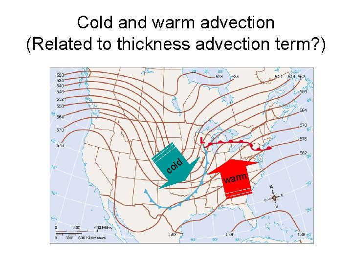
Cold and warm advection (Related to thickness advection term? ) ld o c warm

What about the thickness advection?

Outline • • Waves In Class Problem Quasi-geostrophic Review Vertical Velocity

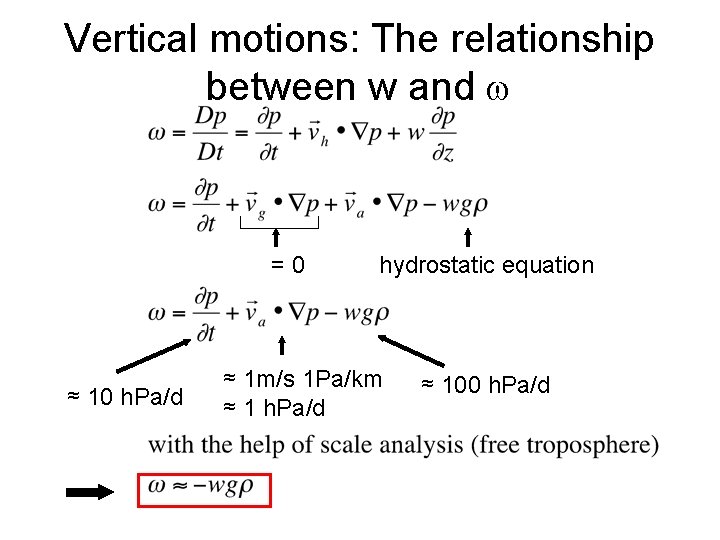
Vertical motions: The relationship between w and =0 ≈ 10 h. Pa/d hydrostatic equation ≈ 1 m/s 1 Pa/km ≈ 1 h. Pa/d ≈ 100 h. Pa/d

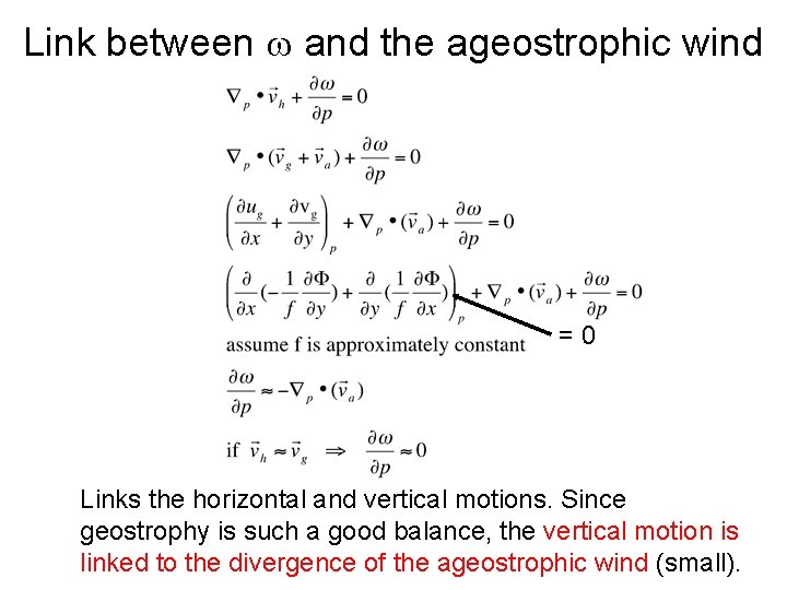
Link between and the ageostrophic wind =0 Links the horizontal and vertical motions. Since geostrophy is such a good balance, the vertical motion is linked to the divergence of the ageostrophic wind (small).

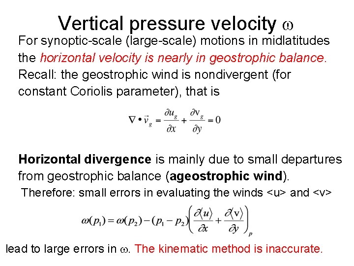
Vertical pressure velocity For synoptic-scale (large-scale) motions in midlatitudes the horizontal velocity is nearly in geostrophic balance. Recall: the geostrophic wind is nondivergent (for constant Coriolis parameter), that is Horizontal divergence is mainly due to small departures from geostrophic balance (ageostrophic wind). Therefore: small errors in evaluating the winds <u> and <v> lead to large errors in . The kinematic method is inaccurate.

Think about this. . . • If I have errors in data, noise. • What happens if you average that data? • What happens if you take an integral over the data? • What happens if you take derivatives of the data?

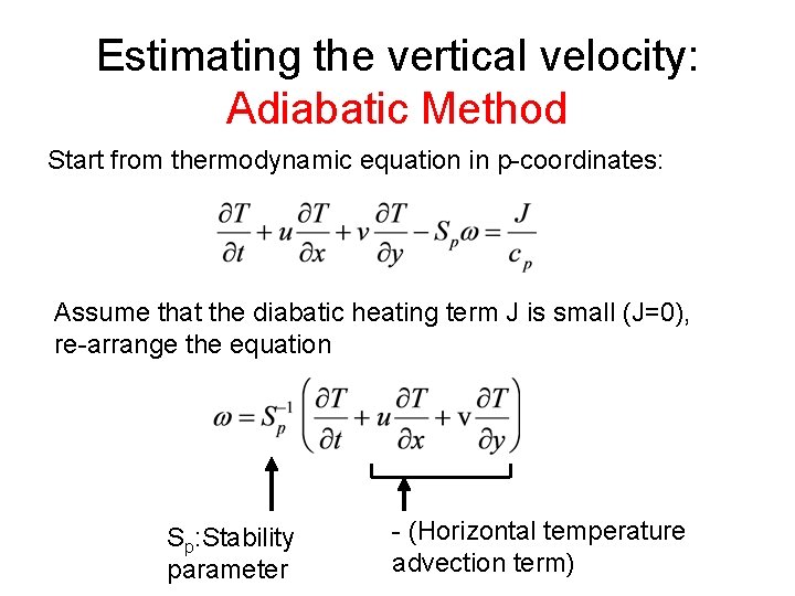
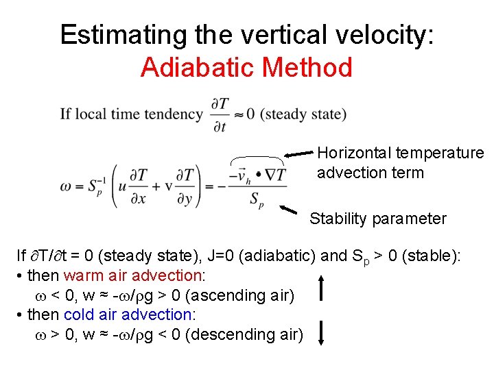
Estimating the vertical velocity: Adiabatic Method Start from thermodynamic equation in p-coordinates: Assume that the diabatic heating term J is small (J=0), re-arrange the equation Sp: Stability parameter - (Horizontal temperature advection term)

Estimating the vertical velocity: Adiabatic Method Horizontal temperature advection term Stability parameter If T/ t = 0 (steady state), J=0 (adiabatic) and Sp > 0 (stable): • then warm air advection: < 0, w ≈ - / g > 0 (ascending air) • then cold air advection: > 0, w ≈ - / g < 0 (descending air)

Adiabatic Method • Based on temperature advection, which is dominated by the geostrophic wind, which is large. Hence this is a reasonable way to estimate local vertical velocity when advection is strong.

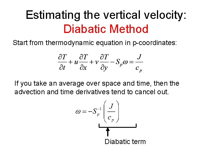
Estimating the vertical velocity: Diabatic Method Start from thermodynamic equation in p-coordinates: If you take an average over space and time, then the advection and time derivatives tend to cancel out. Diabatic term

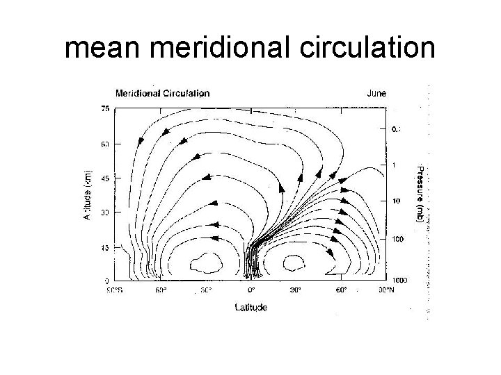
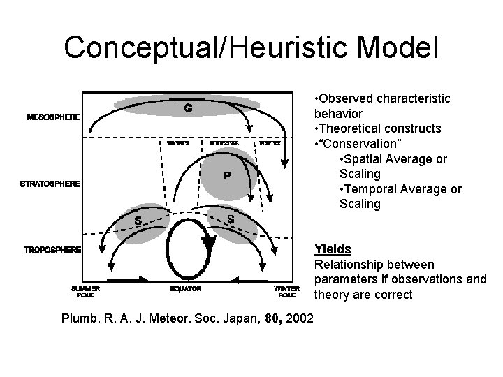
mean meridional circulation

Conceptual/Heuristic Model • Observed characteristic behavior • Theoretical constructs • “Conservation” • Spatial Average or Scaling • Temporal Average or Scaling Yields Relationship between parameters if observations and theory are correct Plumb, R. A. J. Meteor. Soc. Japan, 80, 2002

One more way for vertical velocity

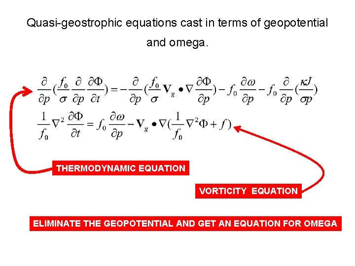
Quasi-geostrophic equations cast in terms of geopotential and omega. THERMODYNAMIC EQUATION VORTICITY EQUATION ELIMINATE THE GEOPOTENTIAL AND GET AN EQUATION FOR OMEGA

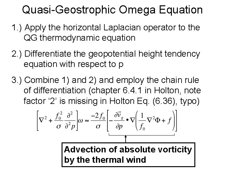
Quasi-Geostrophic Omega Equation 1. ) Apply the horizontal Laplacian operator to the QG thermodynamic equation 2. ) Differentiate the geopotential height tendency equation with respect to p 3. ) Combine 1) and 2) and employ the chain rule of differentiation (chapter 6. 4. 1 in Holton, note factor ‘ 2’ is missing in Holton Eq. (6. 36), typo) Advection of absolute vorticity by thermal wind

Vertical Velocity Summary • Though small, vertical velocity is in some ways the key to weather and climate. It’s important to waves growing and decaying. It is how far away from “balance” the atmosphere is. • It is astoundingly difficult to calculate. If you use all of these methods, they should be equal. But using observations, they are NOT! • In fact, if you are not careful, you will not even to get them to balance in models, because of errors in the numerical approximation.

In Class Problem Solution

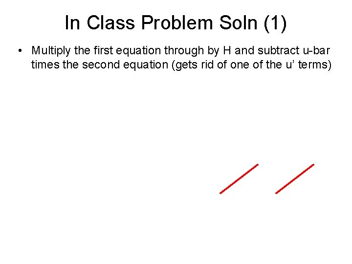
In Class Problem Soln (1) • Multiply the first equation through by H and subtract u-bar times the second equation (gets rid of one of the u’ terms)

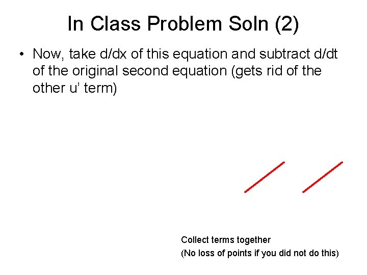
In Class Problem Soln (2) • Now, take d/dx of this equation and subtract d/dt of the original second equation (gets rid of the other u’ term) Collect terms together (No loss of points if you did not do this)

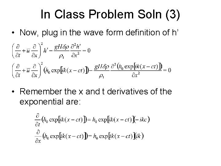
In Class Problem Soln (3) • Now, plug in the wave form definition of h’ • Remember the x and t derivatives of the exponential are:

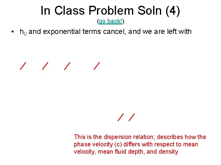
In Class Problem Soln (4) (go back!) • h 0 and exponential terms cancel, and we are left with This is the dispersion relation; describes how the phase velocity (c) differs with respect to mean velocity, mean fluid depth, and density