Anytime Probabilistic Reasoning Rina Dechter Bren School of

Anytime Probabilistic Reasoning Rina Dechter Bren School of Information and Computer Sciences A F B E C D UMD 5/3/2019 Main Collaborators: Alexander Ihler Kalev Kask Radu Marinescu Qi Lou Junkyu Lee 1

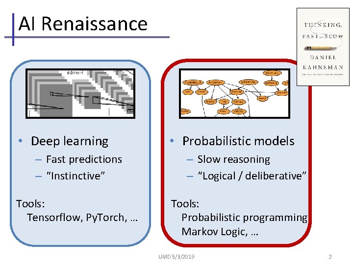
AI Renaissance • Deep learning – Fast predictions – “Instinctive” Tools: Tensorflow, Py. Torch, … • Probabilistic models – Slow reasoning – “Logical / deliberative” Tools: Probabilistic programming, Markov Logic, … UMD 5/3/2019 2

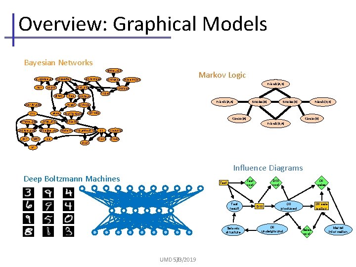
Overview: Graphical Models Bayesian Networks Markov Logic MINVOLSET PULMEMBOLUS KINKEDTUBE INTUBATION VENTMACH DISCONNECT Friends(A, B) PAP SHUNT VENTLUNG MINOVL ANAPHYLAXIS SAO 2 TPR VENITUBE PRESS FIO 2 VENTALV PVSAT ARTCO 2 INSUFFANESTH Friends(A, A) Smokes(B) Smokes(A) Friends(B, B) EXPCO 2 Cancer(A) HYPOVOLEMIA LVEDVOLUME CVP PCWP LVFAILURE STROEVOLUME Cancer(B) CATECHOL Friends(B, A) HISTORY ERRBLOWOUTPUT CO HR HREKG ERRCAUTER HRSAT HRBP BP Influence Diagrams Deep Boltzmann Machines Test cost Test result Seismic structure UMD 5/3/2019 3 Drill cost Drill Oil sales Oil sale policy Oil produced Oil underground Sales cost Market information

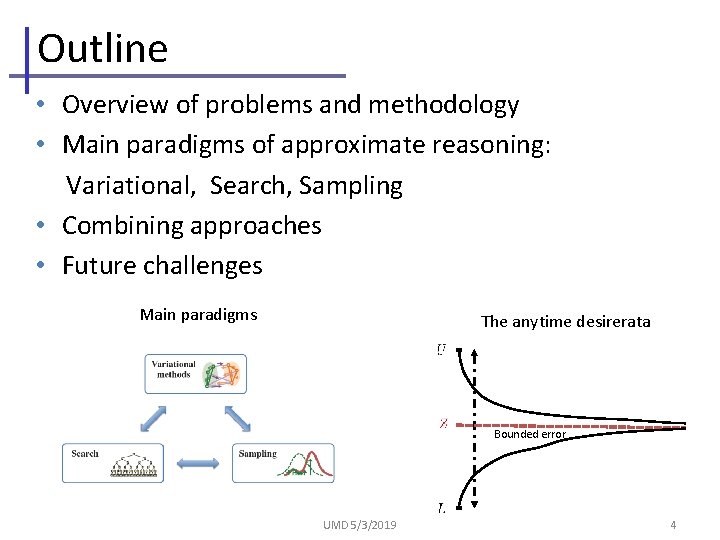
Outline • Overview of problems and methodology • Main paradigms of approximate reasoning: Variational, Search, Sampling • Combining approaches • Future challenges Main paradigms The anytime desirerata Bounded error UMD 5/3/2019 4

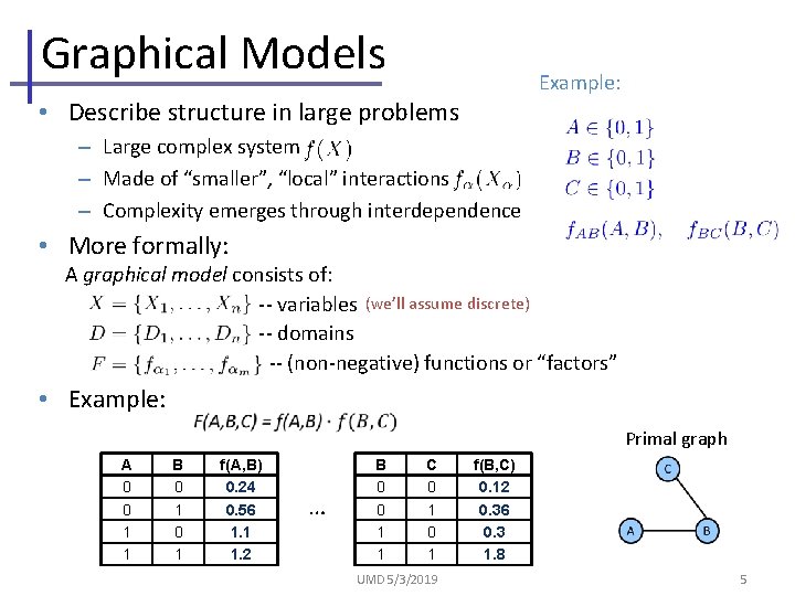
Graphical Models Example: • Describe structure in large problems – Large complex system – Made of “smaller”, “local” interactions – Complexity emerges through interdependence • More formally: A graphical model consists of: -- variables (we’ll assume discrete) -- domains -- (non-negative) functions or “factors” • Example: Primal graph A 0 0 1 1 B 0 1 f(A, B) 0. 24 0. 56 1. 1 1. 2 … B 0 0 1 1 C 0 1 UMD 5/3/2019 f(B, C) 0. 12 0. 36 0. 3 1. 8 5

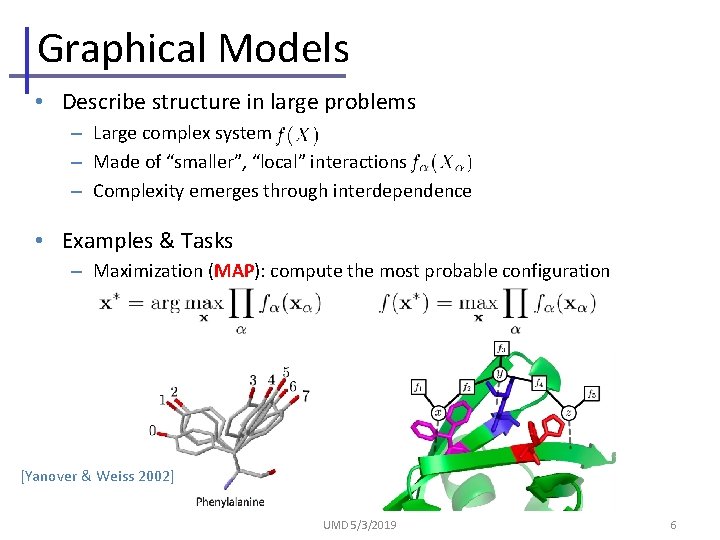
Graphical Models • Describe structure in large problems – Large complex system – Made of “smaller”, “local” interactions – Complexity emerges through interdependence • Examples & Tasks – Maximization (MAP): compute the most probable configuration [Yanover & Weiss 2002] UMD 5/3/2019 6

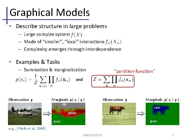
Graphical Models • Describe structure in large problems – Large complex system – Made of “smaller”, “local” interactions – Complexity emerges through interdependence • Examples & Tasks – Summation & marginalization “partition function” and Observation y Marginals p( xi | y ) sky Observation y Marginals p( xi | y ) cow plane grass e. g. , [Plath et al. 2009] UMD 5/3/2019 7

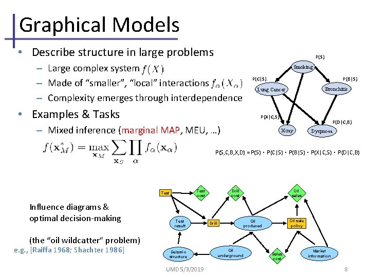
Graphical Models • Describe structure in large problems P(S) – Large complex system – Made of “smaller”, “local” interactions – Complexity emerges through interdependence • Examples & Tasks Smoking P(C|S) P(B|S) Bronchitis Lung Cancer P(X|C, S) – Mixed inference (marginal MAP, MEU, …) P(D|C, B) X-ray Dyspnoea P(S, C, B, X, D) = P(S)・P(C|S)・P(B|S)・P(X|C, S)・P(D|C, B) Test cost Test Influence diagrams & optimal decision-making Test result Drill cost Oil sales Oil sale policy Oil produced Drill (the “oil wildcatter” problem) e. g. , [Raiffa 1968; Shachter 1986] Seismic structure UMD 5/3/2019 Oil underground Sales cost Market information 8

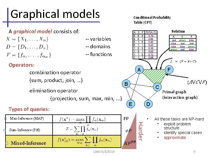
Graphical models Conditional Probability Table (CPT) A graphical model consists of: A 0 0 1 1 -- variables -- domains -- functions Operators: combination operator (sum, product, join, …) Sum-Inference (P(€) � PP Mixed-Inference UMD 5/3/2019 A C F red green blue red blue green red blue Primal graph (interaction graph) D Harder � C E Relation F B Types of queries: Max-Inference (MAP) F P(F|A, C) 0 0. 14 1 0. 96 0 0. 40 1 0. 60 0 0. 35 1 0. 65 0 0. 72 1 0. 68 A elimination operator (projection, sum, max, min, . . . ) � C 0 0 1 1 • All these tasks are NP-hard • exploit problem structure • identify special cases • approximate 9

Example Domains • Natural Language processing – Information extraction, semantic parsing, translation, topic models, … • Computer vision – Object recognition, scene analysis, segmentation, tracking, … • Computational biology – Pedigree analysis, protein folding and binding, sequence matching, … • Networks – Webpage link analysis, social networks, communications, citations, …. • Robotics – Planning & decision making UMD 5/3/2019 10

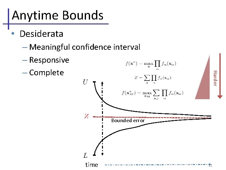
Anytime Bounds • Desiderata Harder – Meaningful confidence interval – Responsive – Complete Bounded error time 11

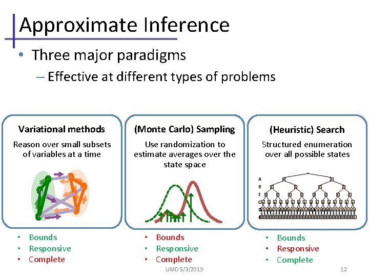
Approximate Inference • Three major paradigms – Effective at different types of problems Variational methods (Monte Carlo) Sampling (Heuristic) Search Reason over small subsets of variables at a time Use randomization to estimate averages over the state space Structured enumeration over all possible states 0 1 A 0 1 B 1 0 1 0 1 E 0 0 1 0 1 C D 0 1 0 1 0 1 0 1 F 010101 0101 01 01010101 010101 • Bounds • Responsive • Complete UMD 5/3/2019 • Bounds • Responsive • Complete 12

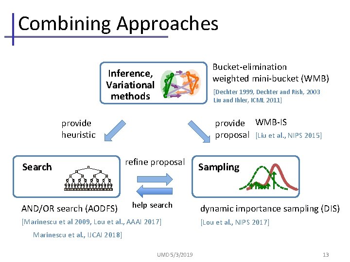
Combining Approaches Bucket-elimination weighted mini-bucket (WMB) Inference, Variational methods [Dechter 1999, Dechter and Rish, 2003 Liu and Ihler, ICML 2011] provide WMB-IS proposal [Liu et al. , NIPS 2015] provide heuristic Search 0 0 refine proposal 1 Sampling 0 1 0 1 0 1 010101010101010101010101 AND/OR search (AODFS) help search [Marinescu et al 2009, Lou et al. , AAAI 2017] dynamic importance sampling (DIS) [Lou et al. , NIPS 2017] Marinescu et al. , IJCAI 2018] UMD 5/3/2019 13

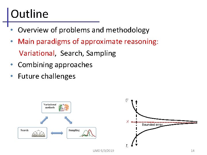
Outline • Overview of problems and methodology • Main paradigms of approximate reasoning: Variational, Search, Sampling • Combining approaches • Future challenges Bounded error UMD 5/3/2019 14

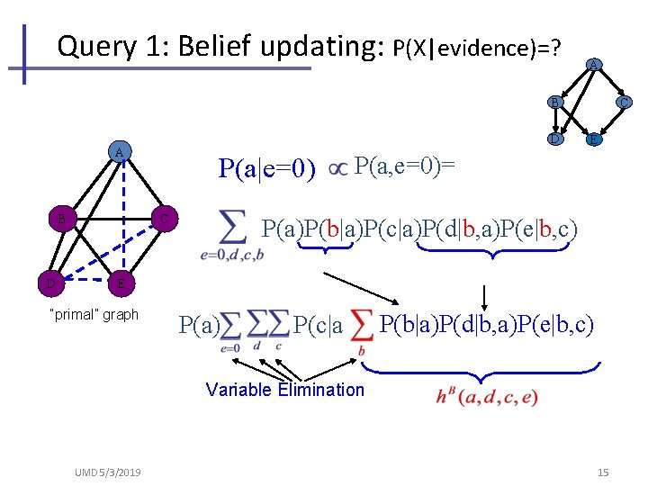
Query 1: Belief updating: P(X|evidence)=? A B D A BB D D P(a|e=0) C C C E P(a, e=0)= P(a)P(b|a)P(c|a)P(d|b, a)P(e|b, c) EE “primal” graph P(a) P(c|a P(b|a)P(d|b, a)P(e|b, c) Variable Elimination UMD 5/3/2019 15

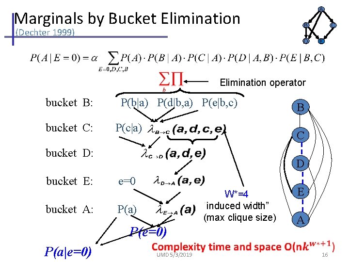
Marginals by Bucket Elimination (Dechter 1999) A B D C E Elimination operator bucket B: bucket C: P(b|a) P(d|b, a) P(e|b, c) P(c|a) C bucket D: bucket E: bucket A: D e=0 W*=4 ”induced width” (max clique size) P(a) P(e=0) P(a|e=0) B UMD 5/3/2019 E A 16

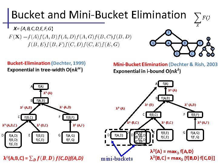
Bucket and Mini-Bucket Elimination X= {A, B, C, D, E, F, G} F A G B A B E C C D A A f(A) C λF (A, B) D f(A, D) f(B, D) f(C, D) 17 F f(B, C) λD (A, B, C) B f(A, B) λC (A, B) f(B, E) f(C, E) λD f(A) G C f(B, F) f(A, G) f(F, G) λF (A, B) f(A, D) D D mini-buckets f(A, D) f(B, D) f(C, D) F f(B, C) λD (B, C) D f(A, B) λC (B) (A) λG (A, F) λE (B, C) E E G λB (A) B D F λG (A, F) λE (B, C) E f(B, E) f(C, E) f(B, F) G f(A, G) f(F, G) λD(A) = max. D f(A, D) λD(B, C) = max. D [f(B, D) f(C, D)]

Bucket and Mini-Bucket Elimination [Dechter 1999; Dechter & Rish, 2003] A summation query; e. g. , partition function A B C D A A f(A) λB (A) B f(A, B) λF (A, B) λC (A, B) C f(B, C) λD (A, B, C) D f(A, D) f(B, D) f(C, D) F f(B, E) f(C, E) λD C f(B, C) λD (B, C) λG (A, F) G f(A, G) f(F, G) λF (A, B) λC (B) (A) f(B, F) λE (B, C) E f(A) D f(A, D) f(B, D) Df(B, D) f(C, D) mini-buckets F λG (A, F) λE (B, C) E f(B, E) f(C, E) f(B, F) G f(A, G) f(F, G) 18 F E G

Bucket and Mini-Bucket Elimination [Dechter 1999; Dechter & Rish, 2003] A maximization query; e. g. , MAP A B F C A G C D A A f(A) B f(A, B) λF (A, B) C f(B, C) λD (A, B, C) D f(A, D) f(B, D) f(C, D) F f(B, E) f(C, E) λD G f(A, G) f(F, G) λF (A, B) λC (B) (A) C f(B, C) f(B, F) λD (B, C) λG (A, F) λE (B, C) E f(A) λB (A) λC (A, B) ED B D f(A, D) D f(B, D) f(C, D) mini-buckets F λG (A, F) λE (B, C) E f(B, E) f(C, E) f(B, F) G f(A, G) f(F, G) 19 F E G

Bucket and Mini-Bucket Elimination [Dechter 1999; Dechter & Rish, 2003, Liu & Ihler 2011] A maximization query; e. g. , MAP F G Assigning MAP value, greedily A A B D E C f(A) λB (A) B f(A, B) λF (A, B) λC (A, B) C f(B, C) λD (A, B, C) D f(A, D) f(B, D) f(C, D) F λG (A, F) λE (B, C) E f(B, E) f(C, E) f(B, F) G f(A, G) f(F, G) UMD 5/3/2019 20

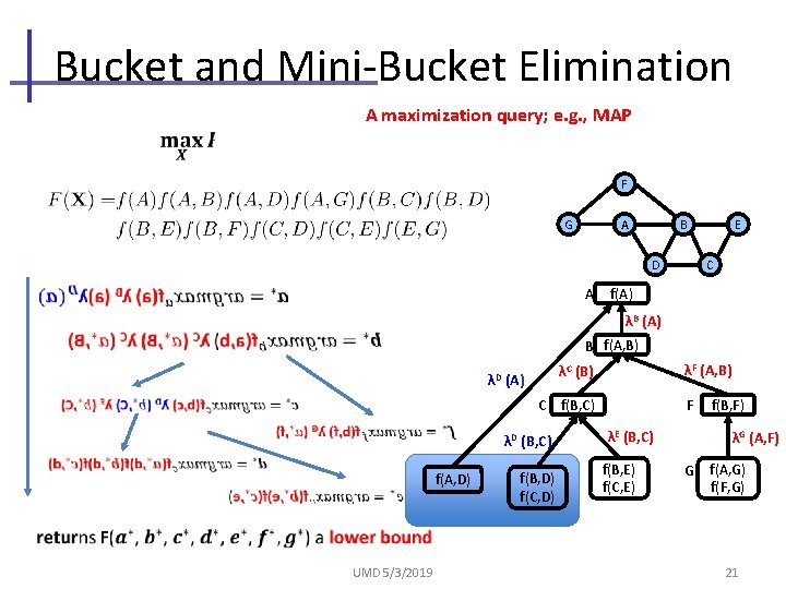
Bucket and Mini-Bucket Elimination A maximization query; e. g. , MAP F A G B C D A E f(A) λB (A) B f(A, B) λD λF (A, B) λC (B) (A) C f(B, C) λD (B, C) f(A, D) UMD 5/3/2019 f(B, D) f(C, D) F λE (B, C) f(B, E) f(C, E) f(B, F) λG (A, F) G f(A, G) f(F, G) 21

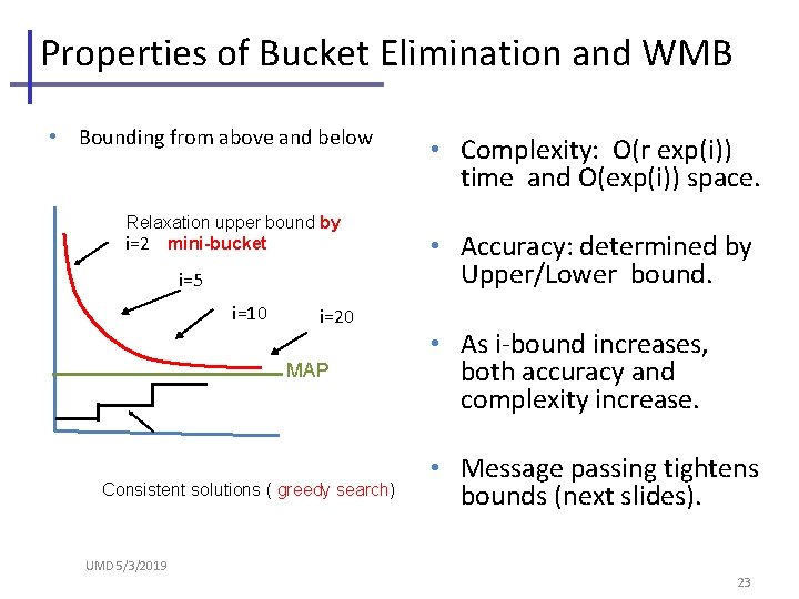
Properties of Bucket Elimination and WMB • Bounding from above and below Relaxation upper bound by i=2 mini-bucket i=5 i=10 i=20 MAP Consistent solutions ( greedy search) • Complexity: O(r exp(i)) time and O(exp(i)) space. • Accuracy: determined by Upper/Lower bound. • As i-bound increases, both accuracy and complexity increase. • Message passing tightens bounds (next slides). UMD 5/3/2019 23

Tightening the Bound; Weighted Mini-Bucket (WMB) [Dechter 2003, Liu & Ihler 2011] A B C D F E G Bounds can be tightened by optimizing weights. F A G • Holder inequality B C D A E f(A) λB (A) B f(A, B) λF (A, B) λC (B) λD (A) C f(B, C) λD (B, C) f(A, D) mini-buckets f(B, D) f(C, D) F λE (B, C) f(B, E) f(C, E) f(B, F) λG (A, F) G f(A, G) f(F, G) 24

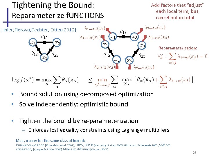
Tightening the Bound: Reparameterize f. UNCTIONS Add factors that “adjust” each local term, but cancel out in total [Ihler, Flerova, Dechter, Otten 2012] Reparameterization: • Bound solution using decomposed optimization • Solve independently: optimistic bound • Tighten the bound by re-parameterization – Enforces lost equality constraints using Lagrange multipliers Many names for the same class of bounds: Dual decomposition [Komodakis et al. 2007], TRW, MPLP [Wainwright et al. 2005; Globerson & Jaakkola 2007, Soft arc consistency [Cooper & Schiex 2004] Max-sum diffusion [Warner 2007] 25

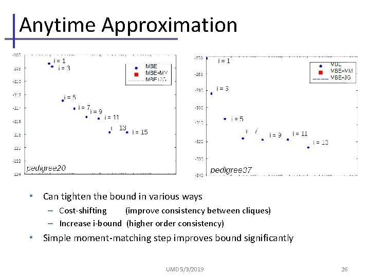
Anytime Approximation • Can tighten the bound in various ways – Cost-shifting (improve consistency between cliques) – Increase i-bound (higher order consistency) • Simple moment-matching step improves bound significantly UMD 5/3/2019 26

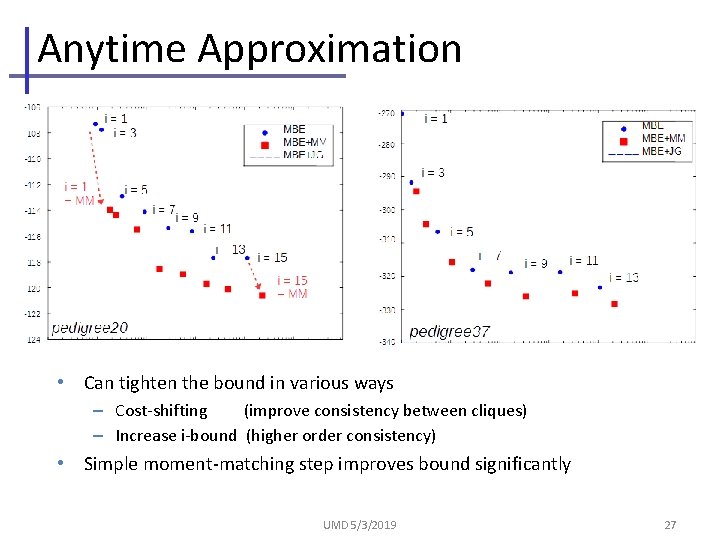
Anytime Approximation • Can tighten the bound in various ways – Cost-shifting (improve consistency between cliques) – Increase i-bound (higher order consistency) • Simple moment-matching step improves bound significantly UMD 5/3/2019 27

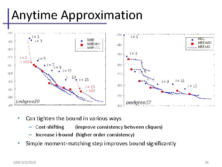
Anytime Approximation • Can tighten the bound in various ways – Cost-shifting (improve consistency between cliques) – Increase i-bound (higher order consistency) • Simple moment-matching step improves bound significantly UMD 5/3/2019 28

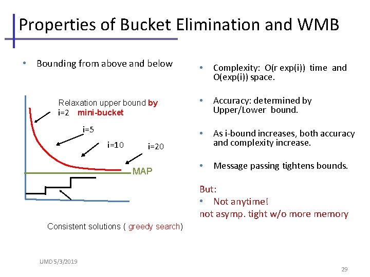
Properties of Bucket Elimination and WMB • Bounding from above and below Relaxation upper bound by i=2 mini-bucket i=5 i=10 • Complexity: O(r exp(i)) time and O(exp(i)) space. • Accuracy: determined by Upper/Lower bound. • As i-bound increases, both accuracy and complexity increase. • Message passing tightens bounds. i=20 MAP But: • Not anytime! not asymp. tight w/o more memory Consistent solutions ( greedy search) UMD 5/3/2019 29

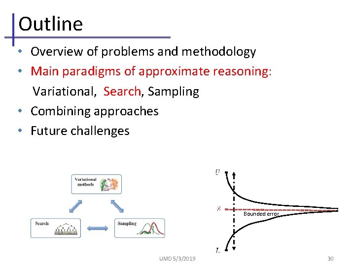
Outline • Overview of problems and methodology • Main paradigms of approximate reasoning: Variational, Search, Sampling • Combining approaches • Future challenges Bounded error UMD 5/3/2019 30

Potential search spaces. A [ ]Pseudo-tree A 0 0 1 1 B 0 1 f 1 2 0 1 4 A 0 0 1 1 C 0 1 f 2 3 0 0 1 A 0 0 1 1 E 0 1 f 3 0 3 2 0 A 0 0 1 1 F 0 1 f 4 2 0 0 2 B 0 0 1 1 C 0 1 f 5 0 1 2 4 B 0 0 1 1 D 0 1 f 6 4 2 1 0 B 0 0 1 1 E 0 1 f 7 3 2 1 0 C 0 0 1 1 D 0 1 f 8 1 4 0 0 E 0 0 1 1 F 0 1 f 9 1 0 0 2 C [A] B [AB] C E [AB] [CB]D F [EA] A D F B E pseudo tree A B C D E F 0 0 1 0 OR 0 tree 1 0 1 A 1 0 0 1 0 1 0 1 B 1 AND/OR 0 1 0 tree 1 OR 0 graph 1 1 0 1 O(n kpw*) O(n 01 01 01 0101 01 01 01 1 1 E O(n)126 nodes OR A O(n) O(n kpw*) 0 1 OR B B 1 0 C OR C E E AND 0 1 0 1 OR AND D D F F 0 1 0 1 0 1 0 0 1 1 1 0 1 0 1 Full AND/OR search tree 54 AND nodes 28 nodes O(n kw*) 1 0 C E 1 Context minimal OR search graph AND 1 0 0 k. F w*) 0 0 1 Full OR search tree memory 1 0 0 C AND/OR 0 D graph 0 1 0 1 time 0 OR AND A 0 1 B B 1 0 C 0 1 0 1 Any query can be computed over any of the search spaces C E 1 0 C E E 0 1 0 1 D D F F 0 1 Context minimal AND/OR search graph 18 AND nodes 6

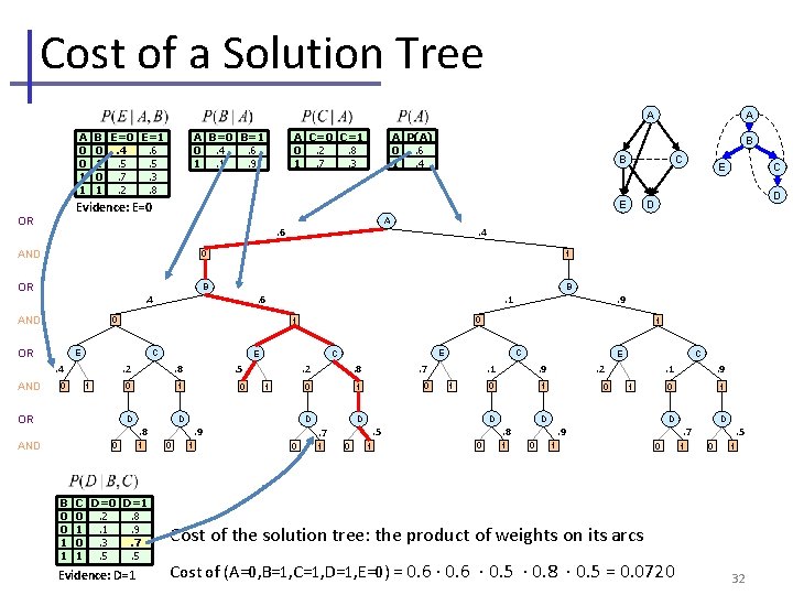
Cost of a Solution Tree A A A 0 0 1 1 A P(A) 0. 6 1. 4 B B A . 6 AND B C . 4 0 1 OR E . 2 . 8 . 5 0 1 0 D D AND 0 B 0 0 1 1 1 C D=0 D=1 0. 2. 8 1. 1. 9 0. 3. 7 1. 5. 5 Evidence: D=1 . 9 0 . 2 . 8 . 7 0 1 0 D . 8 1 C 1 1 . 5 0 E . 1 . 9 0 1 D D . 7 0 1 E C 1 . 9 0 1 E D D B . 1 . 6 0 OR C 1 . 4 AND E . 4 0 OR C E Evidence: E=0 OR AND A C=0 C=1 0. 2. 8 1. 7. 3 A B=0 B=1 0. 4. 6 1. 1. 9 B E=0 E=1 0. 4. 6 1. 5. 5 0. 7. 3 1. 2. 8 1 . 2 0 1 D 1 . 9 0 1 D . 8 0 C . 9 0 1 D . 7 0 1 . 5 0 1 Cost of the solution tree: the product of weights on its arcs Cost of (A=0, B=1, C=1, D=1, E=0) = 0. 6 · 0. 5 · 0. 8 · 0. 5 = 0. 0720 32

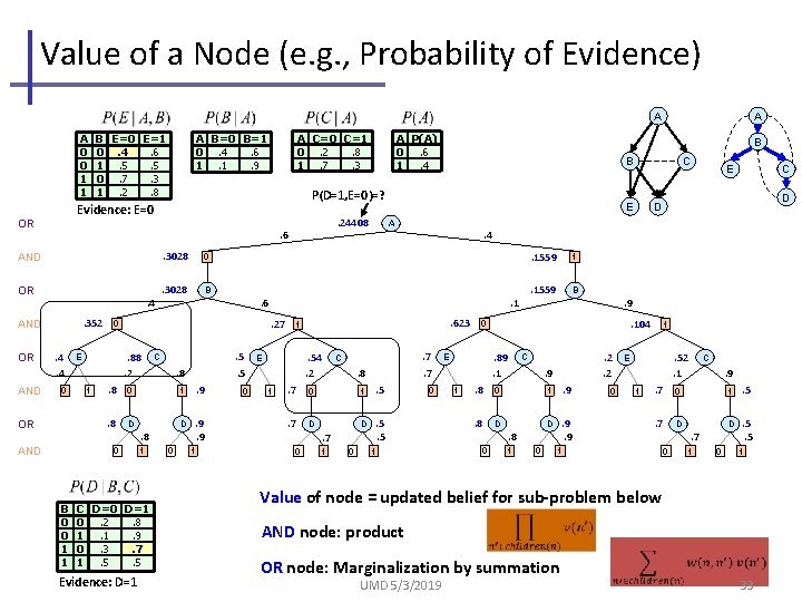
Value of a Node (e. g. , Probability of Evidence) A A A 0 0 1 1 OR . 3028 0 . 3028 B . 4. 352 AND . 24408 . 6 AND . 4. 4 0 OR AND 1 . 8 0 . 8 D 0 B 0 0 1 1 C D=0 D=1 0. 2. 8 1. 1. 9 0. 3. 7 1. 5. 5 Evidence: D=1 . 5. 5 C . 8 1 . 9 D . 9. 9 . 8 1 B A 0 1 0 . 623. 54. 2 1 . 7 0 . 7 D . 7. 7 C . 8 1 . 5 D . 5. 5 . 7 0 1 0 E C D D . 4 1 E C E . 1. 27 . 88. 2 B . 6 0 E A P(A) 0. 6 1. 4 P(D=1, E=0)=? Evidence: E=0 OR OR A C=0 C=1 0. 2. 8 1. 7. 3 A B=0 B=1 0. 4. 6 1. 1. 9 B E=0 E=1 0. 4. 6 1. 5. 5 0. 7. 3 1. 2. 8 0 1 1 . 1559 B . 9. 104 0 . 89. 1 E 1 . 1559 . 8 0 . 8 D 0 . 2. 2 C . 9 1 . 9 D . 9. 9 . 8 1 0 0 1 . 52. 1 E 1 . 7 0 . 7 D 1 0 C . 9 . 7 1 0 1 . 5 D . 5. 5 1 Value of node = updated belief for sub-problem below AND node: product OR node: Marginalization by summation UMD 5/3/2019 33

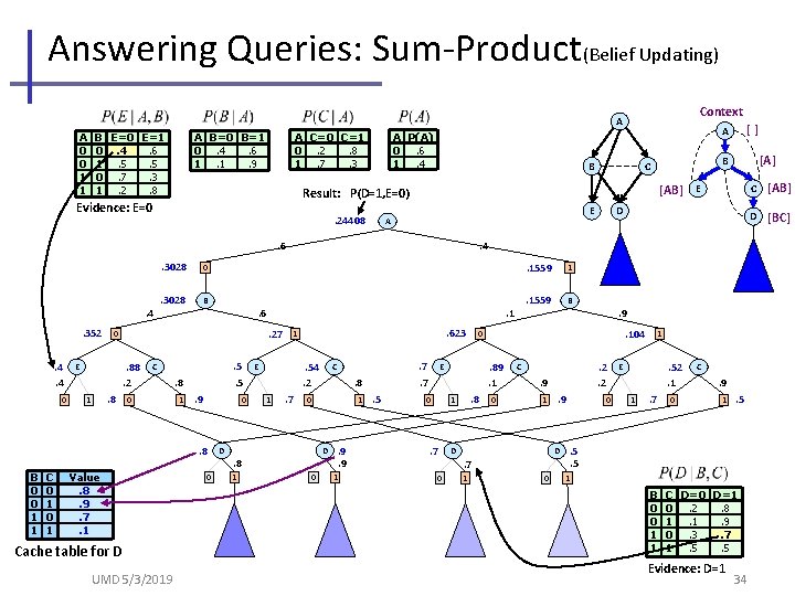
Answering Queries: Sum-Product(Belief Updating) Context A A 0 0 1 1 A C=0 C=1 0. 2. 8 1. 7. 3 A B=0 B=1 0. 4. 6 1. 1. 9 B E=0 E=1 0. 4. 6 1. 5. 5 0. 7. 3 1. 2. 8 A P(A) 0. 6 1. 4 B . 24408 [AB] E E A . 6. 3028 0 . 3028 B . 4. 352. 4. 4 0 . 88. 2 E . 8 1 . 5. 5 C 0 . 8 1 . 9 0 . 8 B 0 0 1 1 C 0 1 . 1. 27 Value. 8. 9. 7. 1 Cache table for D UMD 5/3/2019 0 . 623 1 . 54. 2 E 1 . 7 . 8 1 D . 8 0 . 7. 7 C 0 D 1 D . 4 . 6 0 [A] B C Result: P(D=1, E=0) Evidence: E=0 [] A . 9. 9 1 . 5 . 7 . 1559 B . 8 0 . 2. 2 C . 9 1 D . 9 D . 7 0 . 9. 104 . 89. 1 1 1 0 E 0 . 1559 1 0 0 1 . 52. 1 E 1 . 7 0 C . 9 1 . 5. 5 1 B 0 0 1 1 C D=0 D=1 0. 2. 8 1. 1. 9 0. 3. 7 1. 5. 5 Evidence: D=1 34 C [AB] D [BC]

The Impact of the Pseudo-Tree C K L N O P W=4, h=8 [] H [C] A [CK] [CKLN] [CKO] E J F [CHAE] D [CEJ] M [CD] 0 G [AB] A F [AB] G [AF] [CD] E 0 1 0 A 1 0 N N 0 1 H 1 0 A A 1 0 H M [CD] O N A 1 1 0 A J H 1 E C [CKO] F F 0 1 M M 0101 G G 0101 B B 0101 P A A A A 0 10 10 10 1 [KLO] [ABCJ] (C D K B A O M L N P J H E F G) [CKO] K N O D D D D 010 1 0 1010101 010 1 D M P C [C] [CK] L J J J J 0 1 0 1 1 0 K [ABCD] B B B B B 0 1 0 1 D 01 [C] H 1 L [] L [ABCDJ] L 0 What is a good pseudo-tree? How to find a good one? D [BCD] J 0 L 1 P P P P 0101 [AF] C B 1 0 O O O O E E E E 01 01 01 01 0 1 0 1 (C K H A B E J L N O D P M F G) W=5, h=6 L 1 1 K N N N 0 1 0 1 0 1 [CHA] [CHAB] K 0 [CH] B [CKL] G C 0 [C] F D 01 K 01 M M 0101 O O 01 01 P P P P L L L L 0 10 10 10 10 1 F F 0 10 1 G G 0 10 1 K 01 J J J J 0 10 10 10 10 1 N N N N 0 10 10 10 1 E E E E E E E E 10 10 10 10 10 10 10 10 1 H H H H 0 1 0 10 1 0 10 1 0 1 UMD 5/3/2019 36

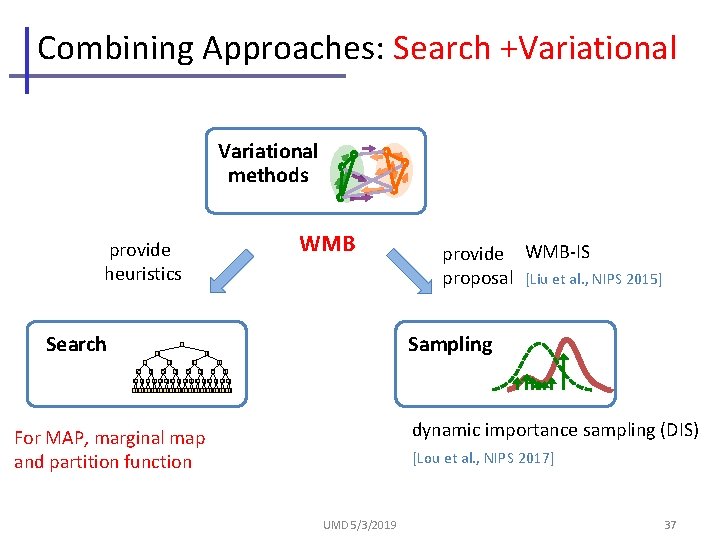
Combining Approaches: Search +Variational methods WMB provide heuristics Search 0 0 provide WMB-IS proposal [Liu et al. , NIPS 2015] Sampling 1 0 1 010101010101010101010101 dynamic importance sampling (DIS) For MAP, marginal map and partition function [Lou et al. , NIPS 2017] UMD 5/3/2019 37

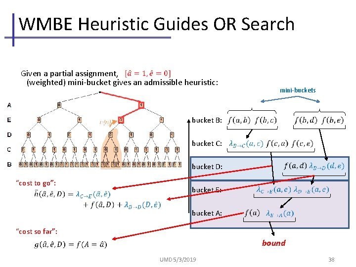
WMBE Heuristic Guides OR Search Given a partial assignment, (weighted) mini-bucket gives an admissible heuristic: mini-buckets bucket B: bucket C: bucket D: “cost to go”: bucket E: bucket A: “cost so far”: bound UMD 5/3/2019 38

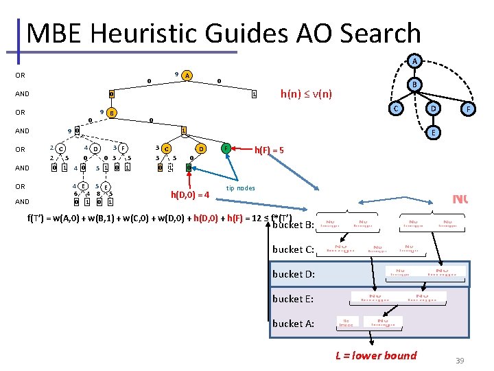
MBE Heuristic Guides AO Search A OR 0 AND 0 OR AND 0 0 OR AND 9 A 9 B 1 4 E 5 E 6 4 8 5 0 1 h(n) ≤ v(n) C D F 0 9 0 2 C 4 D 3 F 5 2 5 0 0 3 0 1 4 0 5 1 0 1 B 1 3 C 3 5 0 1 E D 0 0 h(D, 0) = 4 F h(F) = 5 tip nodes f(T’) = w(A, 0) + w(B, 1) + w(C, 0) + w(D, 0) + h(F) = 12 ≤ f*(T’) bucket B: bucket C: bucket D: bucket E: bucket A: L = lower bound 39

Exploiting Heuristic Search Principles • Weighted Heuristic: [Pohl 1970] f(n)=g(n)+w∙h(n) • Guaranteed w-optimal solution, cost C ≤ w∙C* • Interleaving Best + Depth-First search Upper bound Lower bound Goal: anytime bounds And anytime solution MMAP UMD 5/3/2019 40

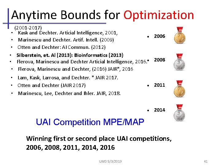
Anytime Bounds for Optimization (2001 -2017) • Kask and Dechter. Articial Intelligence, 2001, 2006 • Marinescu and Dechter. Artif. Intell. (2009) • Otten and Dechter: AI Commun. (2012) • Silberstein, et. Al (2013): Bioinformatics (2013) • Flerova, Marinescu and Dechter Articial Intelligence, 2016. 2008 • Flerova, Marinescu and Dechter, (2016) JAIR", 2016 • Lam, Kask, Larrosa, and Dechter. " JAIR 2017. • Otten and Dechter (JAIR 2017) • Marinescu, Lee, Dechter and Ihler. JAIR, 2018. 2011 2014 UAI Competition MPE/MAP Winning first or second place UAI competitions, 2006, 2008, 2011, 2014, 2016 UMD 5/3/2019 41

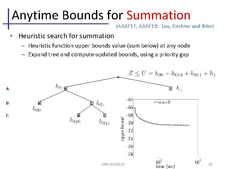
Anytime Bounds for Summation (AAAI’ 17, AAAI’ 18: Lou, Dechter and Ihler) • Heuristic search for summation – Heuristic function upper bounds value (sum below) at any node – Expand tree and compute updated bounds, using a priority gap A B C 0 1 0 1 UMD 5/3/2019 42

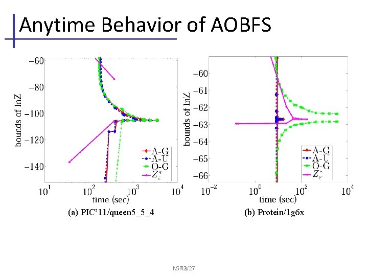
Anytime Behavior of AOBFS (a) PIC’ 11/queen 5_5_4 (b) Protein/1 g 6 x NSF 43 2/27

Anytime Bounds for Marginal MAP [Marinescu, Dechter and Ihler, 2014] A B C MAP variables D E G F SUM variables H constrained pseudo tree C B H F D G 1 B 1 D 0 C D C 1 D C D 0 1 0 1 E E G F 0 1 A mini-buckets B 0 C primal graph pp Complexity: NP complete Not necessarily easy on trees A 0 E 0 1 0 1 0 1 H H 0 1 0 1 h 0 1 UMD 5/3/2019 44

Anytime Solvers for Marginal MAP • Weighted Heuristic: [Lee et. al. AAAI-2016, JAIR 2019] – Weighted Restarting AOBF (WAOBF) – Weighted Restarting RBFAOO (WRBFAOO) – Weighted Repairing AOBF (WRAOBF) Weighted A* search [Pohl 1970] • • non-admissible heuristic Evaluation function: f(n)=g(n)+w∙h(n) • Guaranteed w-optimal solution, cost C ≤ w∙C* • Interleaving Best and depth-first search: (Marinescu et. al AAAI-2017) – Look-ahead (LAOBF), – alternating (AAOBF) Exploiting heuristic search ideas Upper bound Lower bound Goal: anytime bounds And anytime solution MMAP UMD 5/3/2019 45

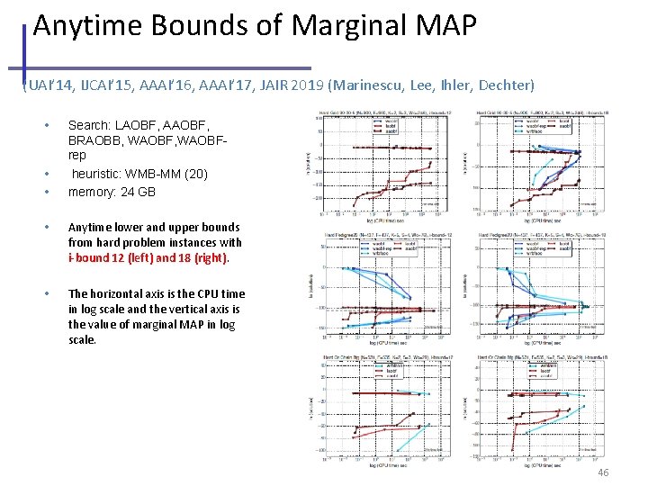
Anytime Bounds of Marginal MAP (UAI’ 14, IJCAI’ 15, AAAI’ 16, AAAI’ 17, JAIR 2019 (Marinescu, Lee, Ihler, Dechter) • • • Search: LAOBF, AAOBF, BRAOBB, WAOBFrep heuristic: WMB-MM (20) memory: 24 GB • Anytime lower and upper bounds from hard problem instances with i-bound 12 (left) and 18 (right). • The horizontal axis is the CPU time in log scale and the vertical axis is the value of marginal MAP in log scale. UMD 5/3/2019 46

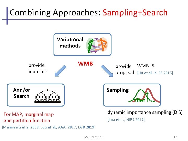
Combining Approaches: Sampling+Search Variational methods WMB provide heuristics And/or Search 0 0 provide WMB-IS proposal [Liu et al. , NIPS 2015] Sampling 1 0 1 010101010101010101010101 dynamic importance sampling (DIS) For MAP, marginal map and partition function [Lou et al. , NIPS 2017] [Marinescu et al 2009, Lou et al. , AAAI 2017, JAIR 2019] NSF 3/27/2019 47

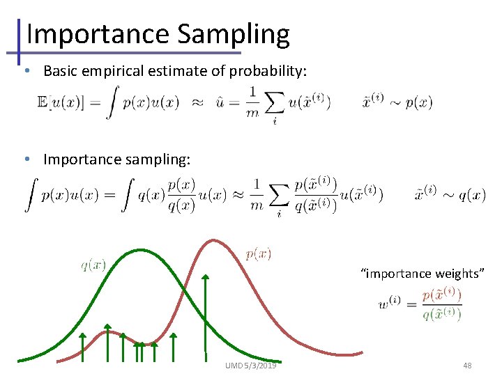
Importance Sampling • Basic empirical estimate of probability: • Importance sampling: “importance weights” UMD 5/3/2019 48

IS on a Bayesian or Markov Network? C • Draw samples from P[A|E=e] directly? D A B F E – Model defines un-normalized p(A, …, E=e) – Build (oriented) tree decomposition & sample B: C: D: E: A: Downward message normalizes bucket; ratio is a conditional distribution Z Can use, WMB, Generalized belief propagation for proposal

Choose a Proposal Combine w Search • • Cutset-Sampling [Bidyuk and Dechter (JAIR, 2007] Build. Ing blocks in current algorithms for Markov Logic Networks • Probabilistic Theorem Proving: Gogate and Domingos, CACM 2016, 2011) ] Sample. Search [Gogate and Dechter. (Artif. Intell. • Lifted Importance Sampling: Venugopal and Gogate, Neur. IPS 2014. AND/OR sampling [Gogate and R. Dechter (Artif. Intell. 2012)] Sampling-based lower bounds [Gogate, Dechter (Intelligenza Artificiale, 2011)] • Dynamic Importance Sampling (DIS) [Lou, Dechter, and Ihler (NIPS 2017)] • Abstraction Sampling [Broka, Dechter, Ihler and Kask (UAI, 2018)]. • Finite-sample Bounds for MMAP [Lou, Dechter, and 2018)] Ihler. (UAI • WMB Importance Sampling (WMB-IS) [Liu, Fisher, Ihler (ICML 2015)] 50

Choosing a proposal- WMB-IS [Liu, Fisher, Ihler 2015] • Can use WMB upper bound to define a proposal mini-buckets B: Weighted mixture: use minibucket 1 with probability w 1 or, minibucket 2 with probability w 2 = 1 - w 1 where C: D: … E: A: Key insight: provides bounded importance weights! UMD 5/3/2019 U = upper bound 51

WMB-IS Bounds [Liu, Fisher, Ihler 2015] • Finite sample bounds on the average • Confidence interval depends on two parts “Empirical Bernstein” bounds – Empirical variance, decreasing as 1/m 1/2 – Upper bound U, decreasing as 1/m -53 -34 -58. 4 -39. 4 -63 -44 BN_6 101 102 103 104 Sample Size (m) 105 BN_11 102 103 104 105 106 Sample Size (m) UMD 5/3/2019 52

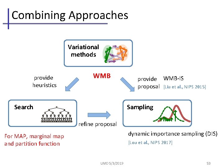
Combining Approaches Variational methods WMB provide heuristics Search 0 0 Sampling 1 0 1 010101010101010101010101 provide WMB-IS proposal [Liu et al. , NIPS 2015] refine proposal dynamic importance sampling (DIS) For MAP, marginal map and partition function [Lou et al. , NIPS 2017] UMD 5/3/2019 53

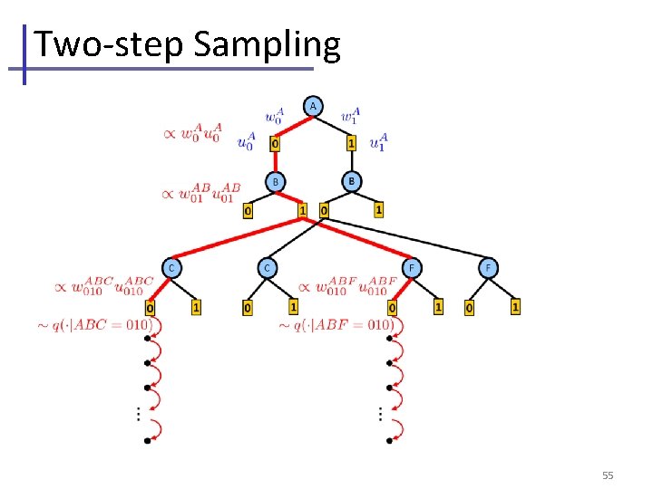
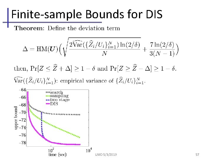
Dynamic Importance Sampling [Lou, Dechter, Ihler, NIPS 2017, AAAI 2019] • Interleave (For partition function) – Building search tree (expand Nd nodes) – Draw samples given search bound (Nl samples) A B C 0 1 0 1 • Key insight: proposal changes (improves) with each step – Use weighted average: better samples get more weight – Derive corresponding concentration bound on Z UMD 5/3/2019 54

Two-step Sampling 55

Finite-sample Bounds for DIS UMD 5/3/2019 57

Individual Results (For partition function) [Lou, Dechter, Ihler, NIPS 2017] UMD 5/3/2019 58

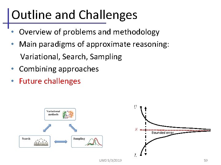
Outline and Challenges • Overview of problems and methodology • Main paradigms of approximate reasoning: Variational, Search, Sampling • Combining approaches • Future challenges Bounded error UMD 5/3/2019 59

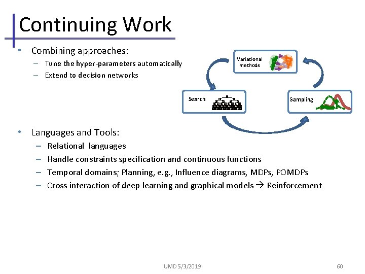
Continuing Work • Combining approaches: Variational methods – Tune the hyper-parameters automatically – Extend to decision networks Search 0 0 1 0 1 010101010101010101010101 Sampling • Languages and Tools: – – Relational languages Handle constraints specification and continuous functions Temporal domains; Planning, e. g. , Influence diagrams, MDPs, POMDPs Cross interaction of deep learning and graphical models Reinforcement UMD 5/3/2019 60

Thank You ! For publication see: http: //www. ics. uci. edu/~dechter/publications. html Alex Ihler Kalev Kask Irina Rish Bozhena Bidyuk Robert Mateescu Radu Marinescu Vibhav Gogate Emma Rollon Lars Otten Natalia Flerova Andrew Gelfand William Lam Junkyu Lee Qi Lou UMD 5/3/2019 61