Antares simulation tools J Brunner CPPM Software scheme

Antares simulation tools J. Brunner CPPM

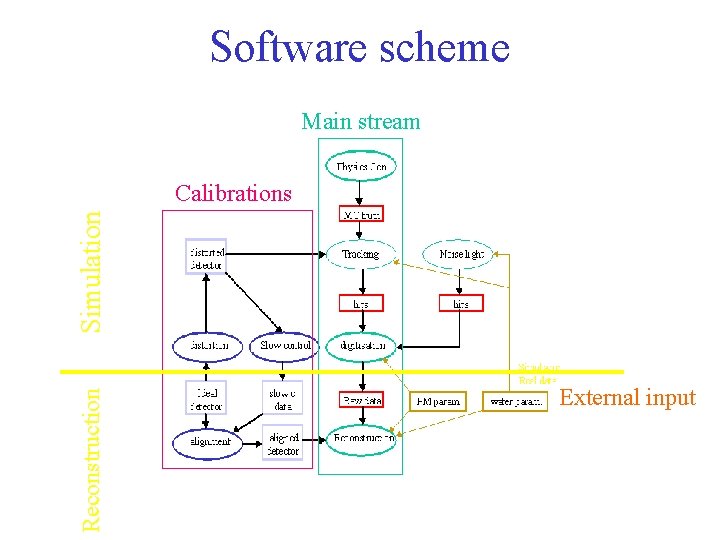
Software scheme Main stream Reconstruction Simulation Calibrations External input

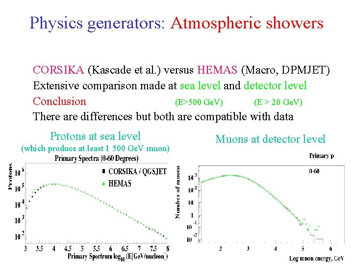
Physics generators: Atmospheric showers CORSIKA (Kascade et al. ) versus HEMAS (Macro, DPMJET) Extensive comparison made at sea level and detector level Conclusion (E>500 Ge. V) (E > 20 Ge. V) There are differences but both are compatible with data Protons at sea level (which produce at least 1 500 Ge. V muon) Muons at detector level

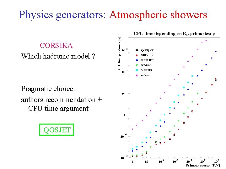
Physics generators: Atmospheric showers CORSIKA Which hadronic model ? Pragmatic choice: authors recommendation + CPU time argument QGSJET

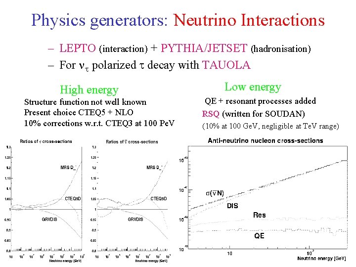
Physics generators: Neutrino Interactions – LEPTO (interaction) + PYTHIA/JETSET (hadronisation) – For polarized decay with TAUOLA High energy Structure function not well known Present choice CTEQ 5 + NLO 10% corrections w. r. t. CTEQ 3 at 100 Pe. V Low energy QE + resonant processes added RSQ (written for SOUDAN) (10% at 100 Ge. V, negligible at Te. V range)

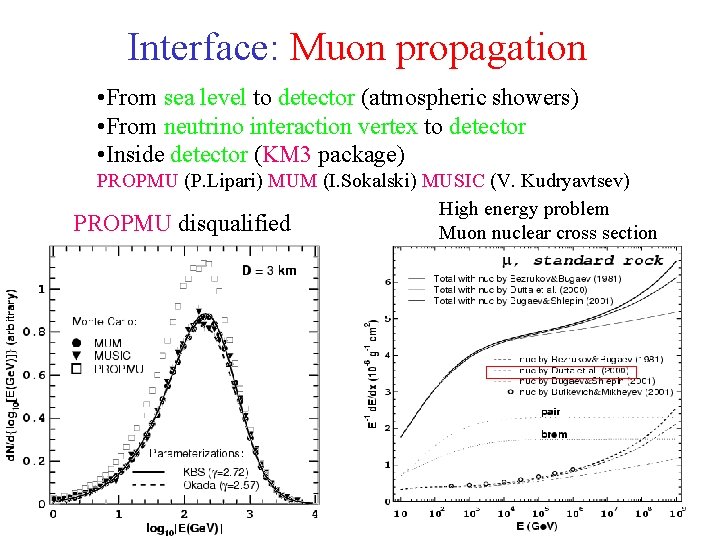
Interface: Muon propagation • From sea level to detector (atmospheric showers) • From neutrino interaction vertex to detector • Inside detector (KM 3 package) PROPMU (P. Lipari) MUM (I. Sokalski) MUSIC (V. Kudryavtsev) High energy problem PROPMU disqualified Muon nuclear cross section

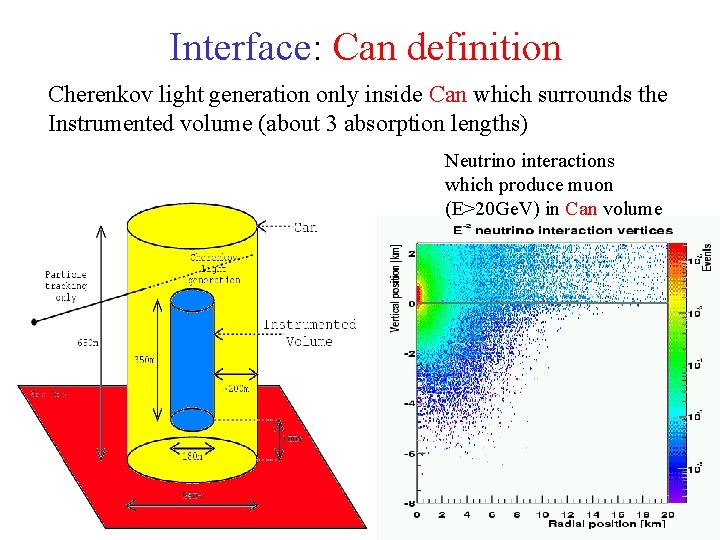
Interface: Can definition Cherenkov light generation only inside Can which surrounds the Instrumented volume (about 3 absorption lengths) Neutrino interactions which produce muon (E>20 Ge. V) in Can volume

Fluxes Many open questions • Cosmic rays • Composition, Spectrum • Atmospheric neutrinos • Spectrum • Contributions from prompt neutrinos • Cosmic neutrinos Needed for precise event numbers Not needed for comparative studies (detector, site, etc) Generic fluxes are sufficient e. g. E-2

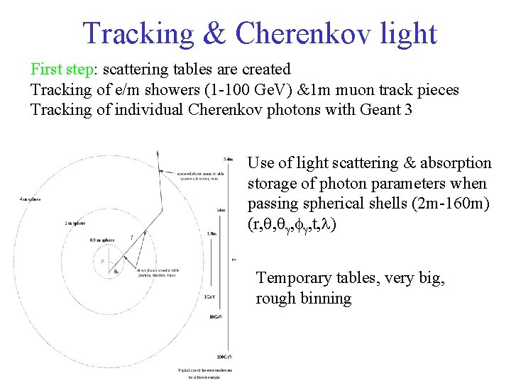
Tracking & Cherenkov light First step: scattering tables are created Tracking of e/m showers (1 -100 Ge. V) &1 m muon track pieces Tracking of individual Cherenkov photons with Geant 3 Use of light scattering & absorption storage of photon parameters when passing spherical shells (2 m-160 m) (r, q, qg, fg, t, l) Temporary tables, very big, rough binning

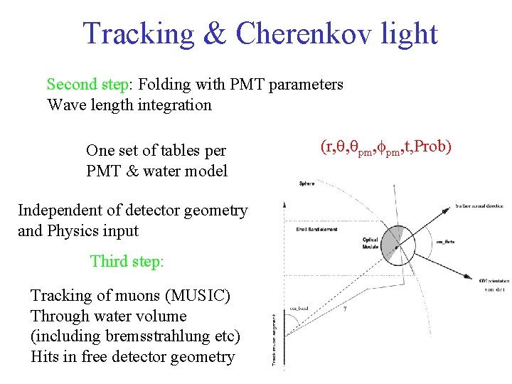
Tracking & Cherenkov light Second step: Folding with PMT parameters Wave length integration One set of tables per PMT & water model Independent of detector geometry and Physics input Third step: Tracking of muons (MUSIC) Through water volume (including bremsstrahlung etc) Hits in free detector geometry (r, q, qpm, fpm, t, Prob)

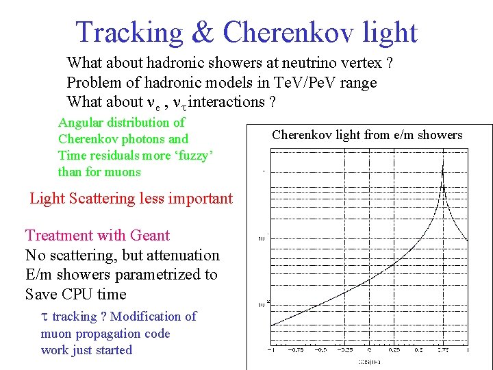
Tracking & Cherenkov light What about hadronic showers at neutrino vertex ? Problem of hadronic models in Te. V/Pe. V range What about e , interactions ? Angular distribution of Cherenkov photons and Time residuals more ‘fuzzy’ than for muons Light Scattering less important Treatment with Geant No scattering, but attenuation E/m showers parametrized to Save CPU time tracking ? Modification of muon propagation code work just started Cherenkov light from e/m showers

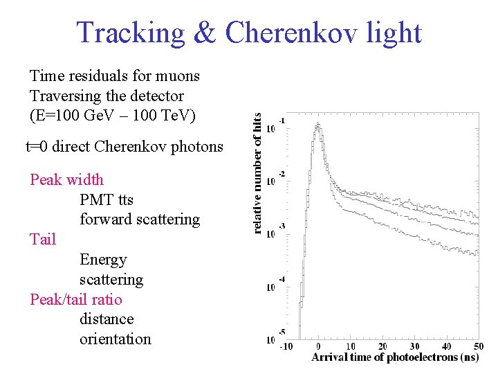
Tracking & Cherenkov light Time residuals for muons Traversing the detector (E=100 Ge. V – 100 Te. V) t=0 direct Cherenkov photons Peak width PMT tts forward scattering Tail Energy scattering Peak/tail ratio distance orientation

Digitisation Full simulation of ARS chip exists as independent package Most analysis done with simplified digitisation: • ignore wave forms • few basic parameters per chip: • integration time • dead time • saturation Results compatible Suggestion for KM 3 simulations: start as well with simplified digitisation (we will not know enough details)

Detector geometry • Defined in external file (ASCII / Oracle) • Basically OM positions & orientations • Not restricted to Antares architecture • Easily adaptable to other concepts • (see work from D. Zaborov)

External inputs Large amount of input parameters/functions needed Physics results depend sensitively on them For comparisons of different simulations they must be under control Earth density PMT/OM characteristics Water parameters

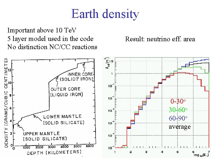
Earth density Important above 10 Te. V 5 layer model used in the code No distinction NC/CC reactions Result: neutrino eff. area 0 -30 o 30 -60 o 60 -90 o average

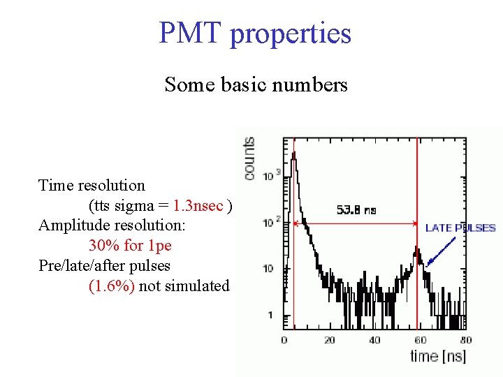
PMT properties Some basic numbers Time resolution (tts sigma = 1. 3 nsec ) Amplitude resolution: 30% for 1 pe Pre/late/after pulses (1. 6%) not simulated

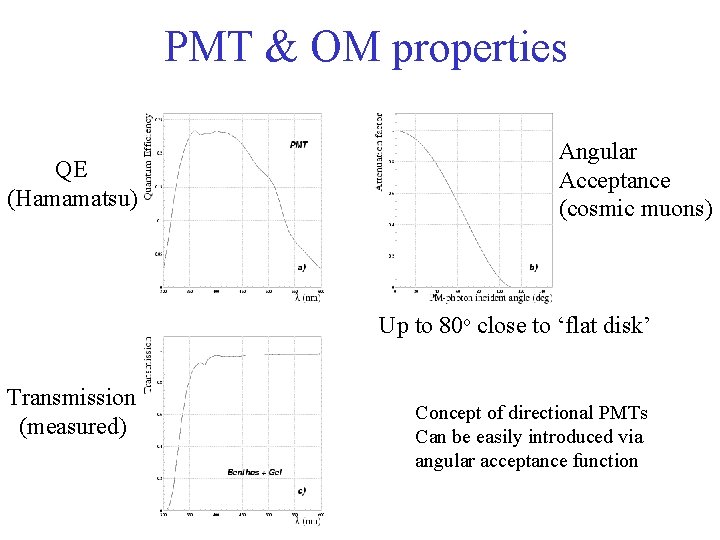
PMT & OM properties QE (Hamamatsu) Angular Acceptance (cosmic muons) Up to 80 o close to ‘flat disk’ Transmission (measured) Concept of directional PMTs Can be easily introduced via angular acceptance function

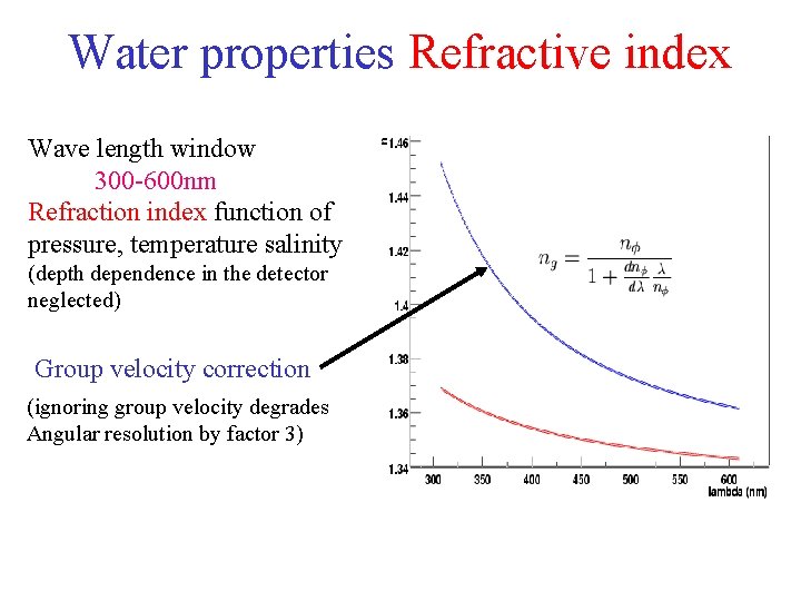
Water properties Refractive index Wave length window 300 -600 nm Refraction index function of pressure, temperature salinity (depth dependence in the detector neglected) Group velocity correction (ignoring group velocity degrades Angular resolution by factor 3)

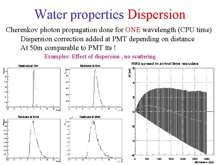
Water properties Dispersion Cherenkov photon propagation done for ONE wavelength (CPU time) Dispersion correction added at PMT depending on distance At 50 m comparable to PMT tts ! Examples: Effect of dispersion , no scattering

Water properties Measurements Summary of measurements at Antares site 220 -300 m Predictions for clean sea water (Rayleigh) 50 -70 m

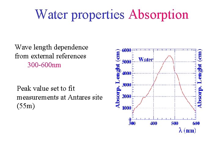
Water properties Absorption Wave length dependence from external references 300 -600 nm Peak value set to fit measurements at Antares site (55 m)

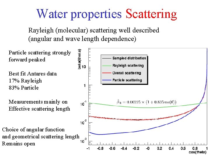
Water properties Scattering Rayleigh (molecular) scattering well described (angular and wave length dependence) Particle scattering strongly forward peaked Best fit Antares data 17% Rayleigh 83% Particle Measurements mainly on Effective scattering length Choice of angular function and geometrical scattering length Remains open

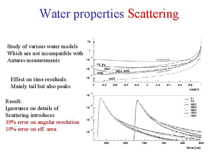
Water properties Scattering Study of various water models Which are not incompatible with Antares measurements Effect on time residuals: Mainly tail but also peaks Result: Ignorance on details of Scattering introduces 30% error on angular resolution 10% error on eff. area

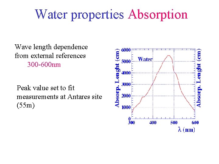
Water properties Absorption Wave length dependence from external references 300 -600 nm Peak value set to fit measurements at Antares site (55 m)

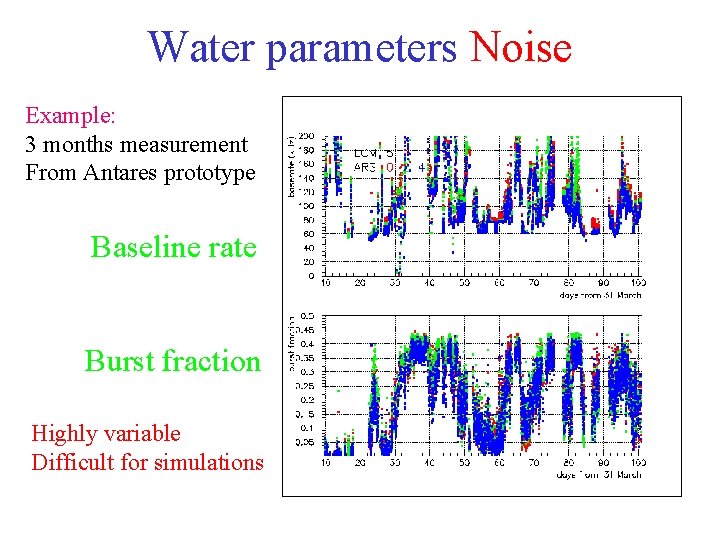
Water parameters Noise Example: 3 months measurement From Antares prototype Baseline rate Burst fraction Highly variable Difficult for simulations

Water parameters Noise • Standard analyses: tunable but constant noise added (most analyses 60 k. Hz – too optimistic ? ) • Standalone noise study: data rate/trigger • Bioluminescence bursts, time/position dependence: studies just started – How to treat effect ? – Fractions of PMTs ‘dead’ (in burst regime) – Individual noise rate per PMT (difficult to ensure stable physics results)

Conclusion • • Full simulation chain operational in Antares External input easily modifiable Scalable to km 3 detectors, different sites Could be used as basis for a km 3 software tool box