ANOVA using SPSS Mathematics Statistics Help University of

ANOVA (using SPSS) Mathematics & Statistics Help University of Sheffield

Learning outcomes • By the end of this session you should: – Understand when to use an analysis of variance – Be able to carry out a one way analysis of variance in SPSS and interpret the output – Be able to conduct a post hoc test to compare differences between groups and interpret the output – Be able to carry out a two way analysis of variance in SPSS and interpret the output – Be able to investigate whethere is an interaction between two categorical explanatory variables in a two way analysis of variance – Be aware of assumptions needed for the analysis of variance model to be valid

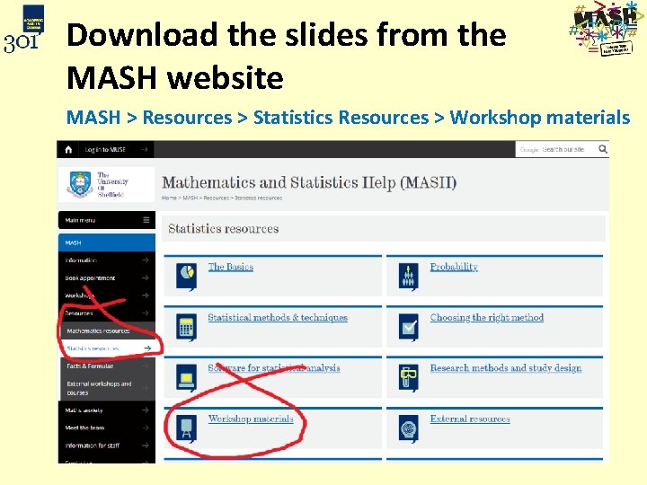
Download the slides from the MASH website MASH > Resources > Statistics Resources > Workshop materials

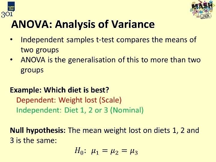
ANOVA: Analysis of Variance

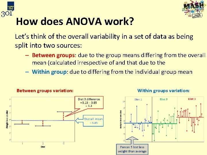
How does ANOVA work? Let’s think of the overall variability in a set of data as being split into two sources: – Between groups: due to the group means differing from the overall mean (calculated irrespective of and that due to the – Within group: due to differing from the individual group mean Between groups variation: Within groups variation:

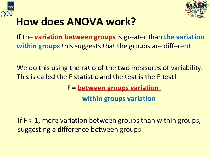
How does ANOVA work? If the variation between groups is greater than the variation within groups this suggests that the groups are different We do this using the ratio of the two measures of variability. This is called the F statistic and the test is the F test! F = between groups variation within groups variation If F > 1, more variation between groups than within groups, suggesting a difference between groups

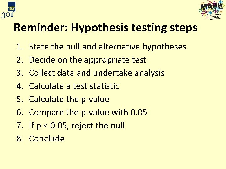
Reminder: Hypothesis testing steps 1. 2. 3. 4. 5. 6. 7. 8. State the null and alternative hypotheses Decide on the appropriate test Collect data and undertake analysis Calculate a test statistic Calculate the p-value Compare the p-value with 0. 05 If p < 0. 05, reject the null Conclude

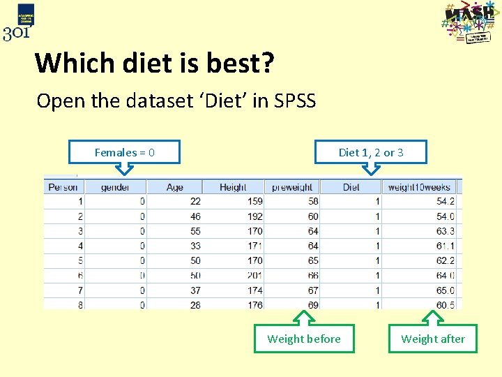
Which diet is best? Open the dataset ‘Diet’ in SPSS Females = 0 Diet 1, 2 or 3 Weight before Weight after

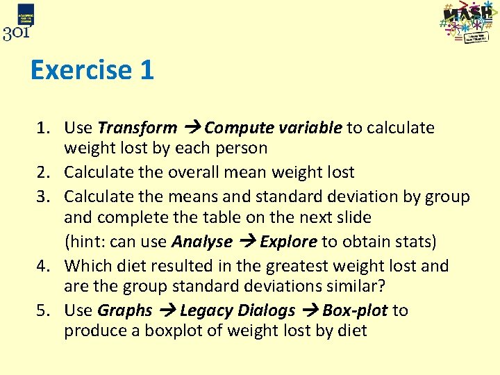
Exercise 1 1. Use Transform Compute variable to calculate weight lost by each person 2. Calculate the overall mean weight lost 3. Calculate the means and standard deviation by group and complete the table on the next slide (hint: can use Analyse Explore to obtain stats) 4. Which diet resulted in the greatest weight lost and are the group standard deviations similar? 5. Use Graphs Legacy Dialogs Box-plot to produce a boxplot of weight lost by diet

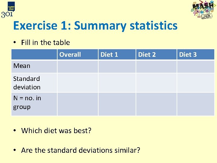
Exercise 1: Summary statistics • Fill in the table Overall Diet 1 Diet 2 Mean Standard deviation N = no. in group • Which diet was best? • Are the standard deviations similar? Diet 3

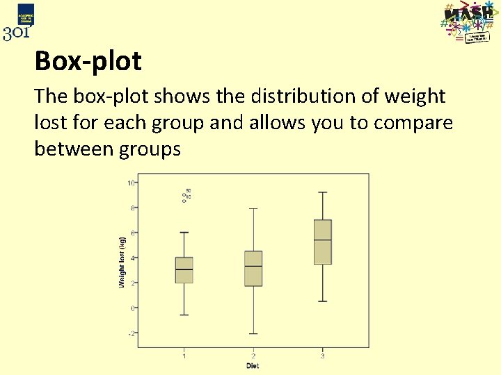
Box-plot The box-plot shows the distribution of weight lost for each group and allows you to compare between groups

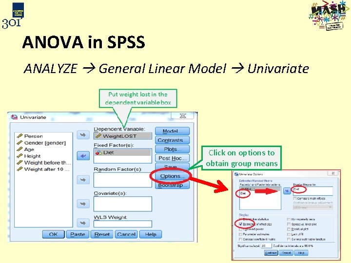
ANOVA in SPSS ANALYZE General Linear Model Univariate Click on options to obtain group means

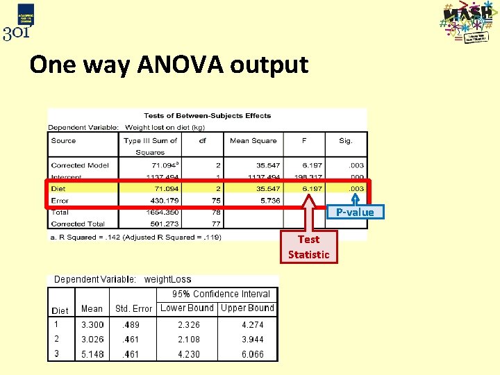
One way ANOVA output P-value Test Statistic

Exercise 2: Discuss the results and how you would interpret the table. Is there a difference between the groups?

Post hoc tests • If there is a significant ANOVA result, pairwise comparisons can be made • They are t-tests with adjustments to control the overall type 1 error rate (reject the null when true): Tukey’s and Scheffe’s tests are the most commonly used post hoc tests Hochberg’s GT 2 is better where the sample sizes for the groups are very different If one group is a control group that you are comparing all others to, use Dunnett’s

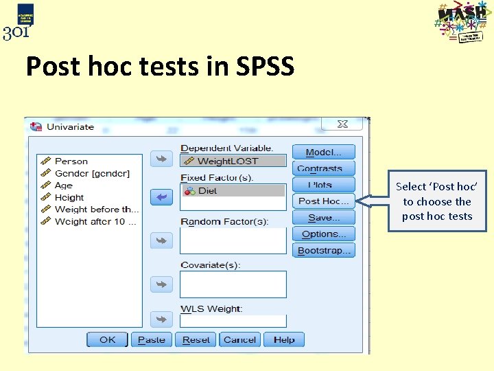
Post hoc tests in SPSS Select ‘Post hoc’ to choose the post hoc tests

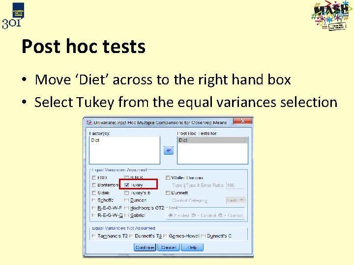
Post hoc tests • Move ‘Diet’ across to the right hand box • Select Tukey from the equal variances selection

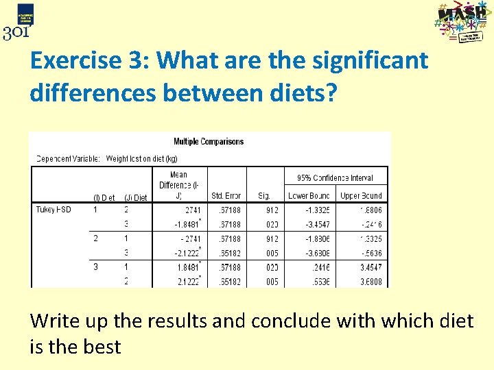
Exercise 3: What are the significant differences between diets? Write up the results and conclude with which diet is the best

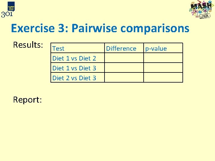
Exercise 3: Pairwise comparisons Results: Report: Test Diet 1 vs Diet 2 Diet 1 vs Diet 3 Diet 2 vs Diet 3 Difference p-value

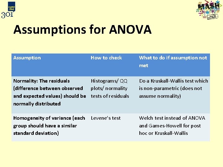
Assumptions for ANOVA Assumption How to check What to do if assumption not met Normality: The residuals Histograms/ QQ (difference between observed plots/ normality and expected values) should be tests of residuals normally distributed Do a Kruskall-Wallis test which is non-parametric (does not assume normality) Homogeneity of variance (each Levene’s test group should have a similar standard deviation) Welch test instead of ANOVA and Games-Howell for post hoc or Kruskall-Wallis

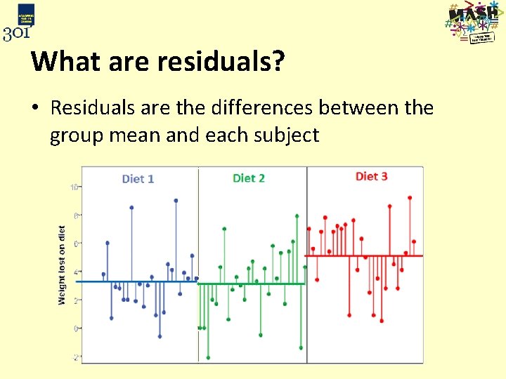
What are residuals? • Residuals are the differences between the group mean and each subject

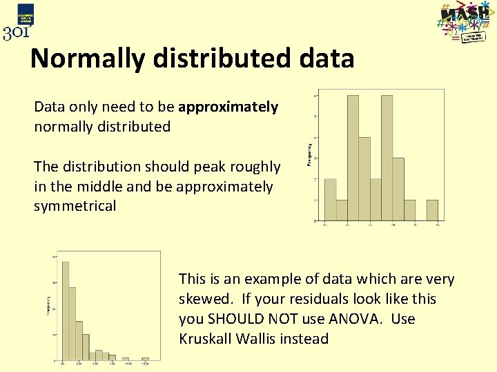
Normally distributed data Data only need to be approximately normally distributed The distribution should peak roughly in the middle and be approximately symmetrical This is an example of data which are very skewed. If your residuals look like this you SHOULD NOT use ANOVA. Use Kruskall Wallis instead

Statistical tests for normality • There are official tests for normality such as the Shapiro-Wilk and Kolmogorov-Smirnoff tests • If p > 0. 05, normality can be assumed Use them with caution: − For small sample sizes (n < 20), the tests are unlikely to detect non-normality − For larger sample sizes (n > 50), the tests can be too sensitive − Very sensitive to outliers Advice: Use histograms, box-plots, comparison of means and medians for assessing normality

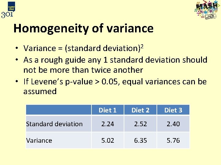
Homogeneity of variance • Variance = (standard deviation)2 • As a rough guide any 1 standard deviation should not be more than twice another • If Levene’s p-value > 0. 05, equal variances can be assumed Diet 1 Diet 2 Diet 3 Standard deviation 2. 24 2. 52 2. 40 Variance 5. 02 6. 35 5. 76

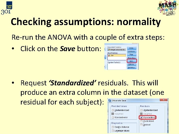
Checking assumptions: normality Re-run the ANOVA with a couple of extra steps: • Click on the Save button: • Request ‘Standardized’ residuals. This will produce an extra column in the dataset (one residual for each subject):

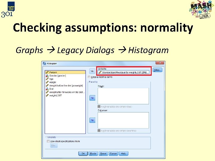
Checking assumptions: normality Graphs Legacy Dialogs Histogram

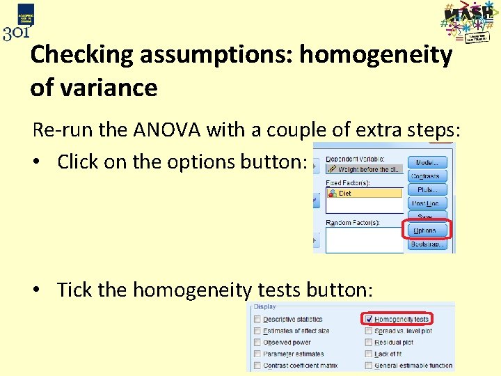
Checking assumptions: homogeneity of variance Re-run the ANOVA with a couple of extra steps: • Click on the options button: • Tick the homogeneity tests button:

Exercise 4: Can normality be assumed? From your histogram of the standardised residuals can normality be assumed? Should you: a) Use ANOVA b) Use Kruskall-Wallis

Exercise 4: Use Levene’s test to examine whether equal variances can be assumed? Null: p= Decision: Reject / do not reject Conclusion:

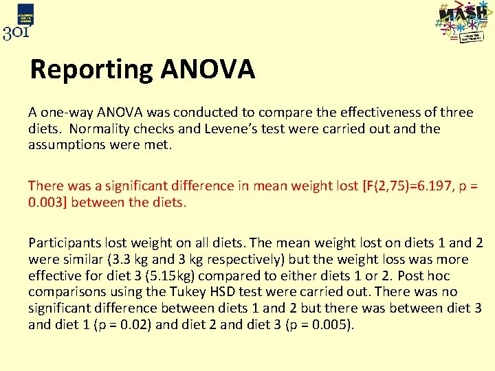
Reporting ANOVA A one-way ANOVA was conducted to compare the effectiveness of three diets. Normality checks and Levene’s test were carried out and the assumptions were met. There was a significant difference in mean weight lost [F(2, 75)=6. 197, p = 0. 003] between the diets. Participants lost weight on all diets. The mean weight lost on diets 1 and 2 were similar (3. 3 kg and 3 kg respectively) but the weight loss was more effective for diet 3 (5. 15 kg) compared to either diets 1 or 2. Post hoc comparisons using the Tukey HSD test were carried out. There was no significant difference between diets 1 and 2 but there was between diet 3 and diet 1 (p = 0. 02) and diet 2 and diet 3 (p = 0. 005).

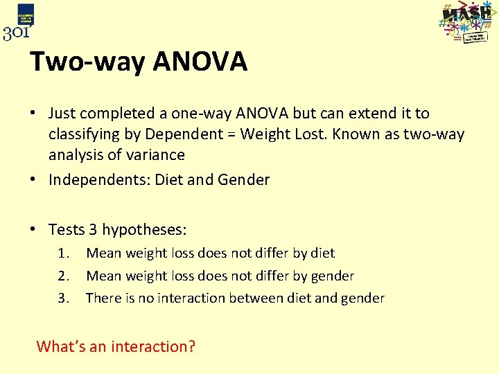
Two-way ANOVA • Just completed a one-way ANOVA but can extend it to classifying by Dependent = Weight Lost. Known as two-way analysis of variance • Independents: Diet and Gender • Tests 3 hypotheses: 1. 2. 3. Mean weight loss does not differ by diet Mean weight loss does not differ by gender There is no interaction between diet and gender What’s an interaction?

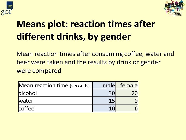
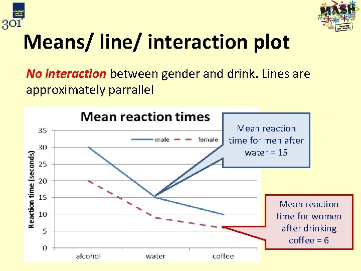
Means plot: reaction times after different drinks, by gender Mean reaction times after consuming coffee, water and beer were taken and the results by drink or gender were compared Mean reaction time (seconds) alcohol water coffee male female 30 20 15 9 10 6

Means/ line/ interaction plot No interaction between gender and drink. Lines are approximately parrallel Mean reaction time for men after water = 15 Mean reaction time for women after drinking coffee = 6

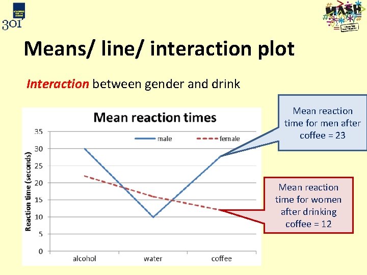
Means/ line/ interaction plot Interaction between gender and drink Mean reaction time for men after coffee = 23 Mean reaction time for women after drinking coffee = 12

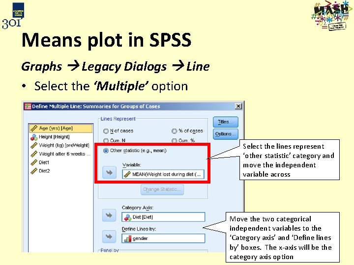
Means plot in SPSS Graphs Legacy Dialogs Line • Select the ‘Multiple’ option Select the lines represent ‘other statistic’ category and move the independent variable across Move the two categorical independent variables to the ‘Category axis’ and ‘Define lines by’ boxes. The x-axis will be the category axis option

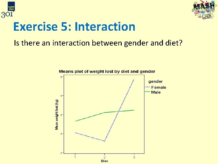
Exercise 5: Interaction Is there an interaction between gender and diet?

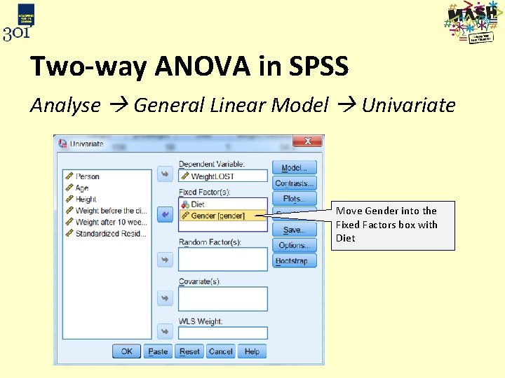
Two-way ANOVA in SPSS Analyse General Linear Model Univariate Move Gender into the Fixed Factors box with Diet

Exercise 6: Two way ANOVA with interaction • Run a two way ANOVA for gender and diet. Don’t forget to click on the Options box and request the estimated marginal means for Diet and Gender • Check the assumptions – Levene’s test for homogeneity of variance / look at the SDs within each group – Save the residuals and plot them – does they look normally distributed • Are the main effects of gender and diet significant? • Is the interaction between the two significant?

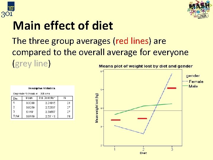
Main effect of diet The three group averages (red lines) are compared to the overall average for everyone (grey line)

What if there is a significant interaction? • The main effects need to be discussed by group e. g. for males/ females separately • The best way to describe what is happening is by using the means plot • Separate ANOVA’s can be carried out by group e. g. testing diet by gender

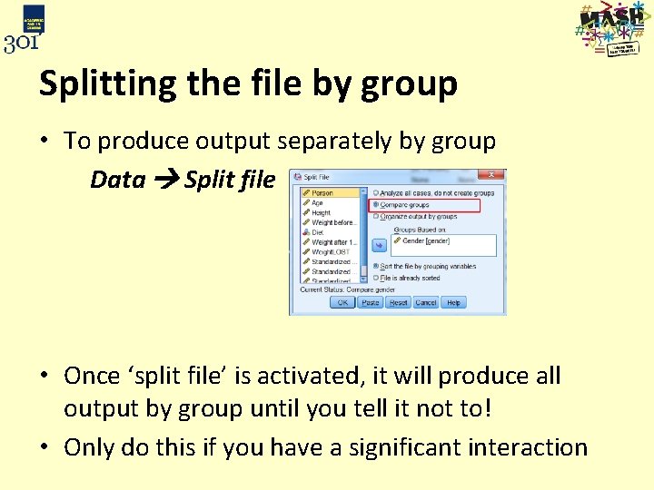
Splitting the file by group • To produce output separately by group Data Split file • Once ‘split file’ is activated, it will produce all output by group until you tell it not to! • Only do this if you have a significant interaction

Exercise 7: ANOVA by gender • Split the file by group as described on the previous slide • Run the ANOVA again (removing gender from the Fixed Factor list) • Is there a diet effect for males and/ or females? • If there is, what is it and which diets are different?

Exercise 7: Post hoc tests and reporting results If the ANOVA is significant, produce suitable post hoc tests and summarise differences using summary statistics by diet/ gender

Learning outcomes You should now: – Understand when to use an analysis of variance – Be able to carry out a one way analysis of variance in SPSS and interpret the output – Be able to conduct a post hoc test to compare differences between groups and interpret the output – Be able to carry out a two way analysis of variance in SPSS and interpret the output – Be able to investigate whethere is an interaction between two categorical explanatory variables in a two way analysis of variance – Be aware of assumptions needed for the analysis of variance model to be valid

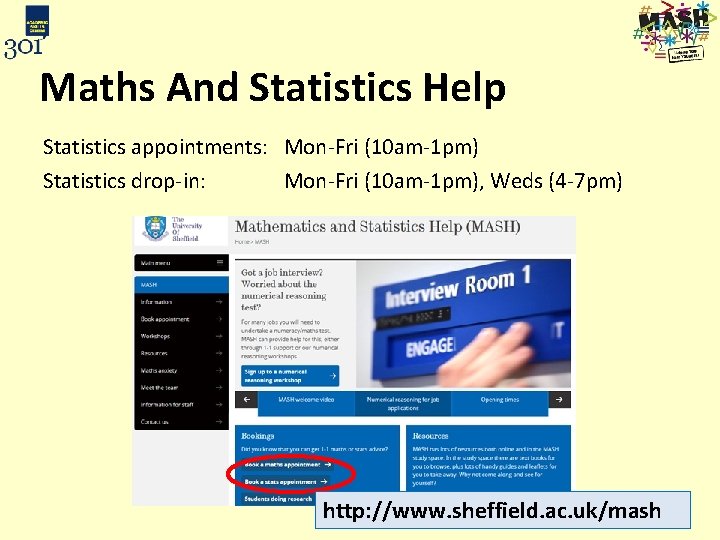
Maths And Statistics Help Statistics appointments: Mon-Fri (10 am-1 pm) Statistics drop-in: Mon-Fri (10 am-1 pm), Weds (4 -7 pm) http: //www. sheffield. ac. uk/mash

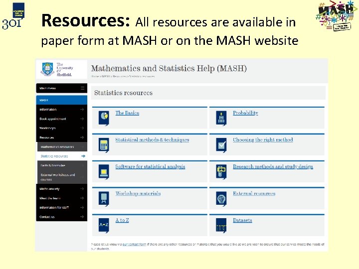
Resources: All resources are available in paper form at MASH or on the MASH website

Contacts Staff Jenny Freeman (j. v. freeman@sheffield. ac. uk) Basile Marquier (b. marquier@sheffield. ac. uk) Marta Emmett (m. emmett@sheffield. ac. uk) Website http: //www. sheffield. ac. uk/mash Follow MASH on twitter: @mash_uos