ANOVA PSY 440 June 26 2008 Clarification Null

ANOVA PSY 440 June 26, 2008

Clarification: Null & Alternative Hypotheses • Sometimes the null hypothesis is that some value is zero (e. g. , difference between groups), or that groups are equal • Sometimes the null hypothesis is the opposite of what you are “hoping” or “expecting” to find based on theory • It is usually (if not always) that “nothing interesting, special, or unusual is going on here. ” • If you are confused, look for the “nothing special” hypothesis, and that is usually H 0

Clarification: Null & Alternative Hypotheses • Examples of the “nothing special” H 0 – These proportions aren’t unusual, they are what previous literature has typically found. There’s nothing unusual about my sample (could be that proportions are equal or unequal, depends on what constitutes “nothing special”) – The mean score in my sample isn’t unusual - it is no different from the mean I would expect, based on what I know about the population (could be that the expected mean is 0, could be that it is some positive or negative number - depends on what constitutes “nothing special”) – The two groups have equal means - nothing special about the experimental condition (this is the more intuitive scenario) • Sometimes you “want” to reject H 0, other times you are more interested in “ruling out” unexpected alternatives.

Review: Assumptions of the t-test • Each of the population distributions follows a normal curve • The two populations have the same variance • If the variance is not equal, but the sample sizes are equal or very close, you can still use a t-test • If the variance is not equal and the samples are very different in size, use the corrected degrees of freedom provided after Levene’s test (see spss output)

Using spss to conduct t-tests • One-sample t-test: Analyze =>Compare Means =>One sample t-test. Select the variable you want to analyze, and type in the expected mean based on your null hypothesis. • Paired or related samples t-test: Analyze =>Compare Means =>Paired samples t-test. Select the variables you want to compare and drag them into the “pair 1” boxes labeled “variable 1” and “variable 2” • Independent samples t-test: Analyze =>Compare Means =>Independent samples t-test. Specify test variable and grouping variable, and click on define groups to specify how grouping variable will identify groups.

Using excel to compute t-tests • =t-test(array 1, array 2, tails, type) • Select the arrays that you want to compare, specify number of tails (1 or 2) and type of t -test (1=dependent, 2=independent w/equal variance assumed, 3=independent w/unequal variance assumed). • Returns the p-value associated with the ttest.

t-tests and the General Linear Model • Think of grouping variable as x and “test variable” as y in a regression analysis. Does knowing what group a person is in help you predict their score on y? • If you code the grouping variable as a binary numeric variable (e. g. , group 1=0 and group 2=1), and run a regression analysis, you will get similar results as you would get in an independent samples t-test! (try it and see for yourself)

Conceptual Preview of ANOVA • Thinking in terms of the GLM, the t-test is telling you how big the variance or difference between the two groups is, compared to the variance in your y variable (between vs. within group variance). • In terms of regression, how much can you reduce “error” (or random variability) by looking at scores within groups rather than scores for the entire sample?

Effect Size for t Test for Independent Means • Estimated effect size after a completed study

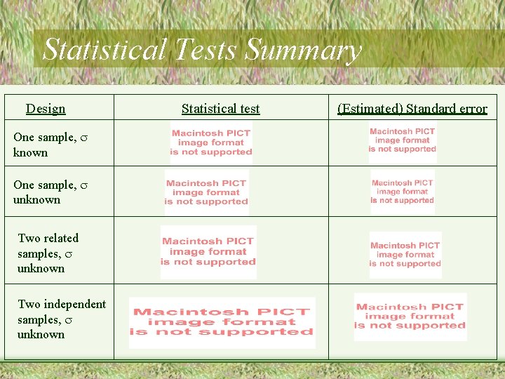
Statistical Tests Summary Design One sample, known One sample, unknown Two related samples, unknown Two independent samples, unknown Statistical test (Estimated) Standard error

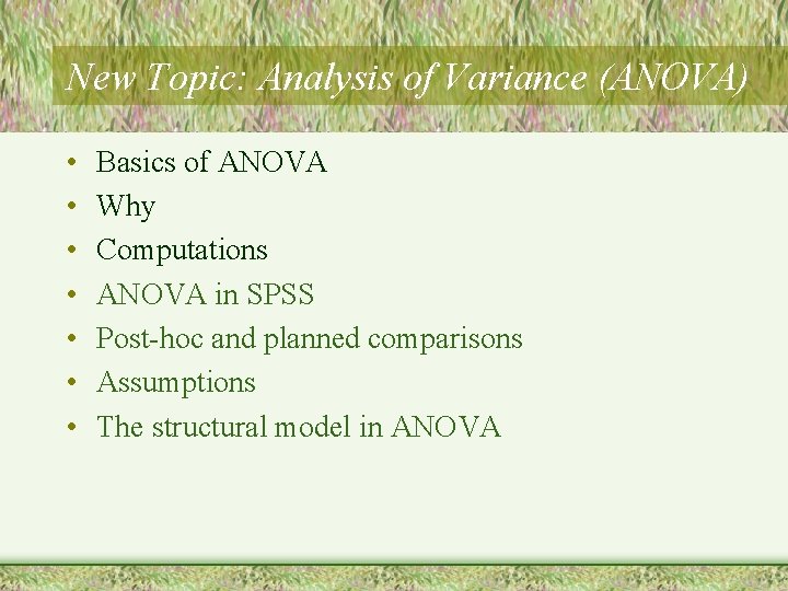
New Topic: Analysis of Variance (ANOVA) • • Basics of ANOVA Why Computations ANOVA in SPSS Post-hoc and planned comparisons Assumptions The structural model in ANOVA

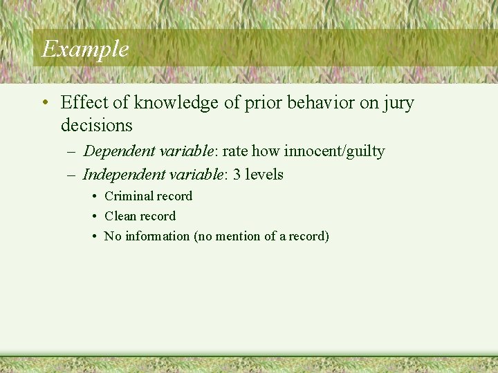
Example • Effect of knowledge of prior behavior on jury decisions – Dependent variable: rate how innocent/guilty – Independent variable: 3 levels • Criminal record • Clean record • No information (no mention of a record)

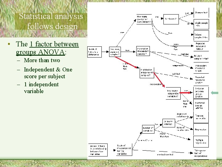
Statistical analysis follows design • The 1 factor between groups ANOVA: – More than two – Independent & One score per subject – 1 independent variable

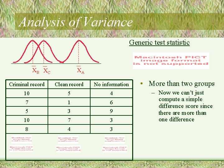
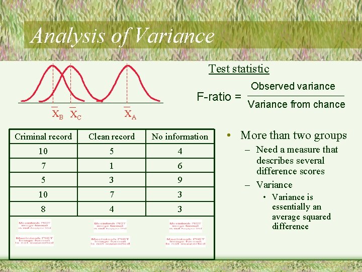
Analysis of Variance Generic test statistic XB XC XA Criminal record Clean record No information 10 5 4 7 1 6 5 3 9 10 7 3 8 4 3 • More than two groups – Now we can’t just compute a simple difference score since there are more than one difference

Analysis of Variance Test statistic F-ratio = XB XC XA Criminal record Clean record No information 10 5 4 7 1 6 5 3 9 10 7 3 8 4 3 Observed variance Variance from chance • More than two groups – Need a measure that describes several difference scores – Variance • Variance is essentially an average squared difference

Testing Hypotheses with ANOVA • Hypothesis testing: a five step program – Step 1: State your hypotheses • Null hypothesis (H 0) – All of the populations all have same mean • Alternative hypotheses (HA) – Not all of the populations all have same mean – There are several alternative hypotheses – We will return to this issue later

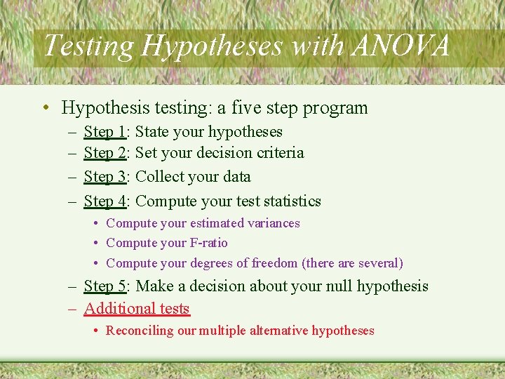
Testing Hypotheses with ANOVA • Hypothesis testing: a five step program – – Step 1: State your hypotheses Step 2: Set your decision criteria Step 3: Collect your data Step 4: Compute your test statistics • Compute your estimated variances • Compute your F-ratio • Compute your degrees of freedom (there are several) – Step 5: Make a decision about your null hypothesis – Additional tests • Reconciling our multiple alternative hypotheses

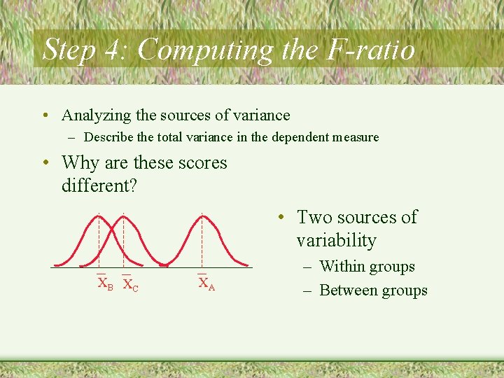
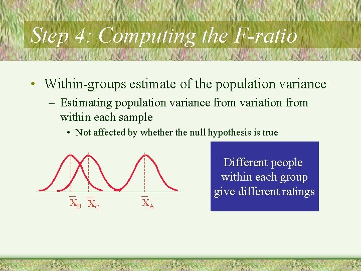
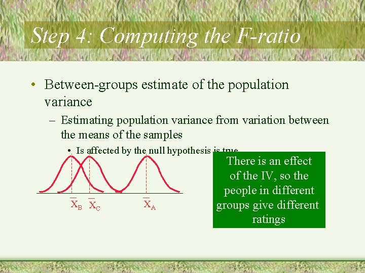
Step 4: Computing the F-ratio • Analyzing the sources of variance – Describe the total variance in the dependent measure • Why are these scores different? • Two sources of variability XB XC XA – Within groups – Between groups

Step 4: Computing the F-ratio • Within-groups estimate of the population variance – Estimating population variance from variation from within each sample • Not affected by whether the null hypothesis is true XB XC XA Different people within each group give different ratings

Step 4: Computing the F-ratio • Between-groups estimate of the population variance – Estimating population variance from variation between the means of the samples • Is affected by the null hypothesis is true XB XC XA There is an effect of the IV, so the people in different groups give different ratings

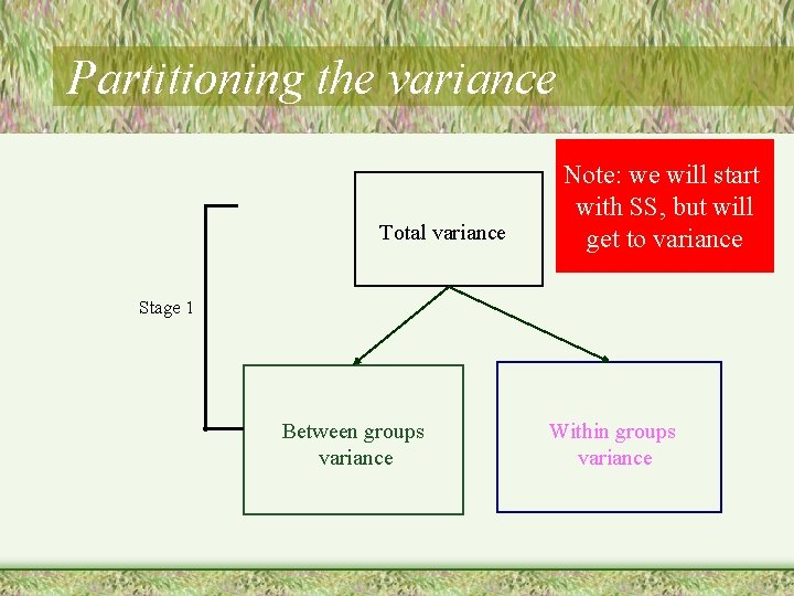
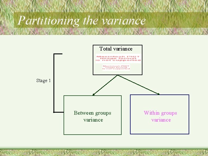
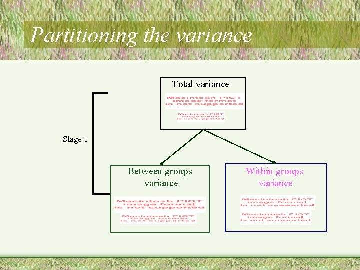
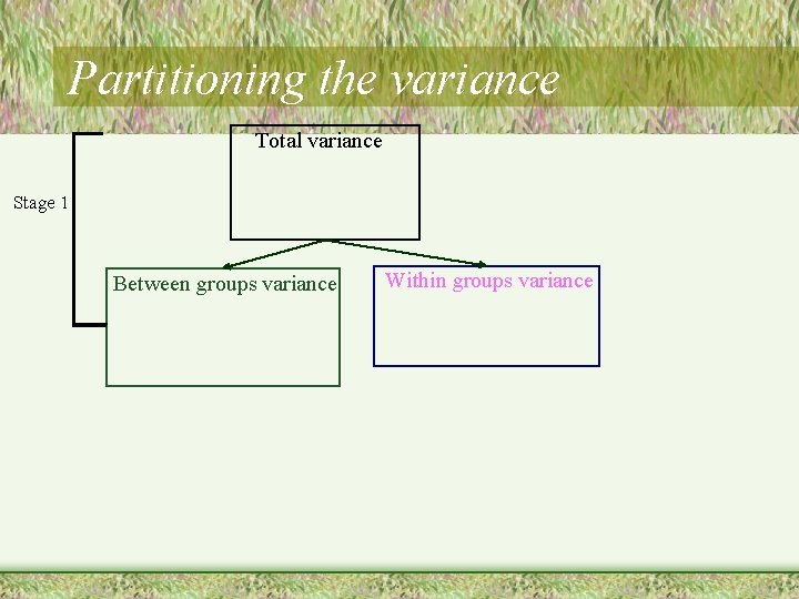
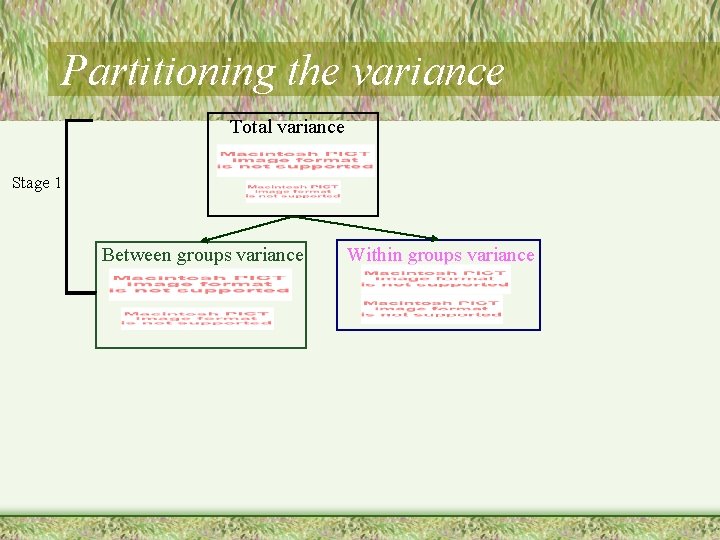
Partitioning the variance Total variance Note: we will start with SS, but will get to variance Stage 1 Between groups variance Within groups variance

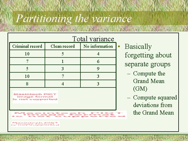
Partitioning the variance Total variance Criminal record Clean record No information 10 5 4 7 1 6 5 3 9 10 7 3 8 4 3 • Basically forgetting about separate groups – Compute the Grand Mean (GM) – Compute squared deviations from the Grand Mean

Partitioning the variance Total variance Stage 1 Between groups variance Within groups variance

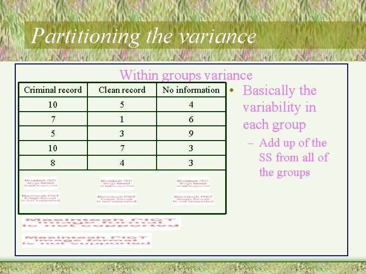
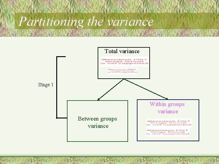
Partitioning the variance Criminal record 10 7 5 Within groups variance Clean record No information • Basically the 5 4 variability in 1 6 each group 3 9 10 7 3 8 4 3 – Add up of the SS from all of the groups

Partitioning the variance Total variance Stage 1 Within groups variance Between groups variance

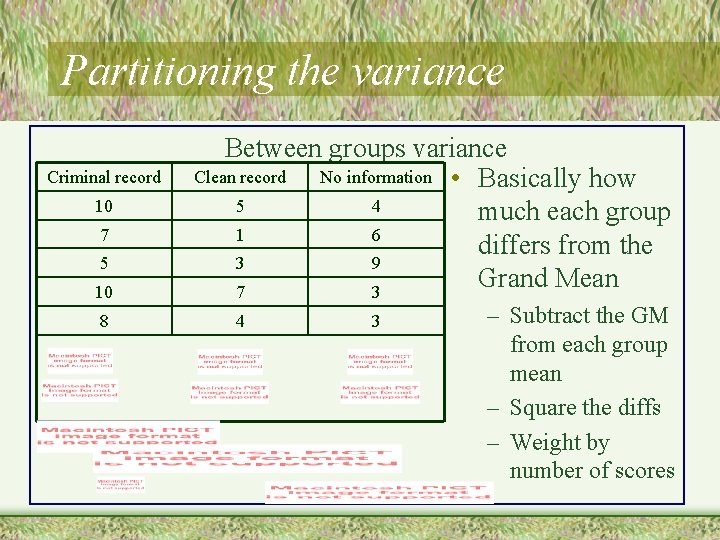
Partitioning the variance Criminal record 10 7 5 10 8 Between groups variance Clean record No information • Basically how 5 4 much each group 1 6 differs from the 3 9 Grand Mean 7 3 4 3 – Subtract the GM from each group mean – Square the diffs – Weight by number of scores

Partitioning the variance Total variance Stage 1 Between groups variance Within groups variance

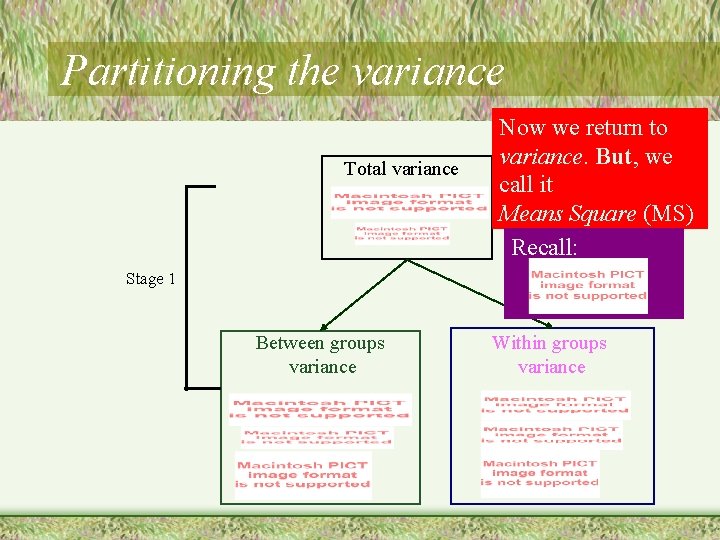
Partitioning the variance Total variance Now we return to variance. But, we call it Means Square (MS) Recall: Stage 1 Between groups variance Within groups variance

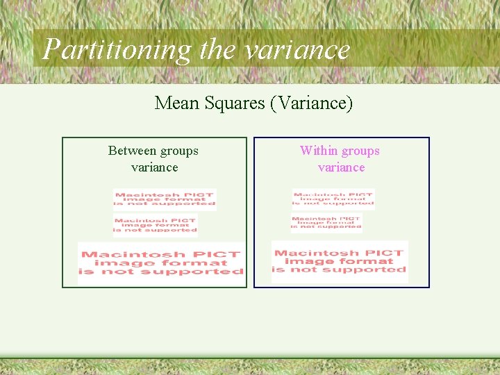
Partitioning the variance Mean Squares (Variance) Between groups variance Within groups variance

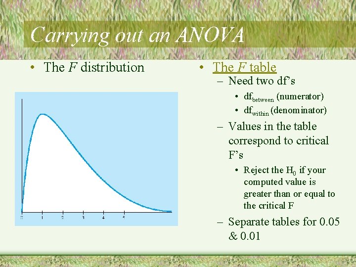
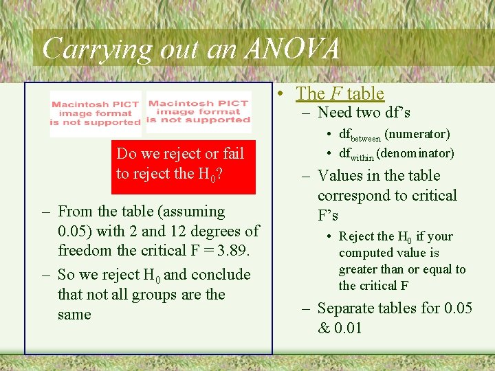
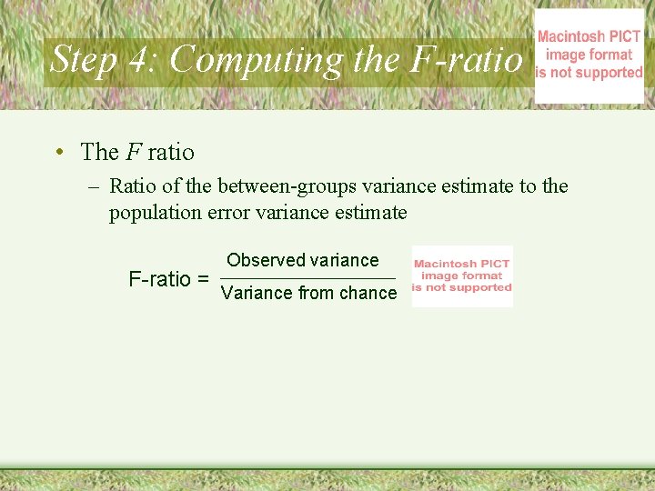
Step 4: Computing the F-ratio • The F ratio – Ratio of the between-groups to the within-groups population variance estimate F-ratio = Observed variance Variance from chance • The F distribution • The F table Do we reject or fail to reject the H 0?

Carrying out an ANOVA • The F distribution • The F table – Need two df’s • dfbetween (numerator) • dfwithin (denominator) – Values in the table correspond to critical F’s • Reject the H 0 if your computed value is greater than or equal to the critical F – Separate tables for 0. 05 & 0. 01

Carrying out an ANOVA • The F table – Need two df’s Do we reject or fail to reject the H 0? – From the table (assuming 0. 05) with 2 and 12 degrees of freedom the critical F = 3. 89. – So we reject H 0 and conclude that not all groups are the same • dfbetween (numerator) • dfwithin (denominator) – Values in the table correspond to critical F’s • Reject the H 0 if your computed value is greater than or equal to the critical F – Separate tables for 0. 05 & 0. 01

Assumptions in ANOVA • Populations follow a normal curve • Populations have equal variances

Planned Comparisons • Reject null hypothesis – Population means are not all the same • Planned comparisons – Within-groups population variance estimate – Between-groups population variance estimate • Use the two means of interest – Figure F in usual way

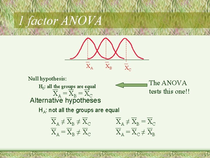
1 factor ANOVA XA XB XC Null hypothesis: The ANOVA tests this one!! H 0: all the groups are equal XA = X B = X C Alternative hypotheses HA: not all the groups are equal XA ≠ X B ≠ X C XA = X B ≠ X C XA ≠ X B = X C XA = X C ≠ X B

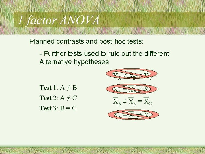
1 factor ANOVA Planned contrasts and post-hoc tests: - Further tests used to rule out the different Alternative hypotheses XA ≠ X B ≠ X C Test 1: A ≠ B Test 2: A ≠ C Test 3: B = C XA = X B ≠ X C XA ≠ X B = X C XA = X C ≠ X B

Planned Comparisons • Simple comparisons • Complex comparisons • Bonferroni procedure – Use more stringent significance level for each comparison

Controversies and Limitations • Omnibus test versus planned comparisons – Conduct specific planned comparisons to examine • Theoretical questions • Practical questions – Controversial approach

ANOVA in Research Articles • F(3, 67) = 5. 81, p <. 01 • Means given in a table or in the text • Follow-up analyses – Planned comparisons • Using t tests

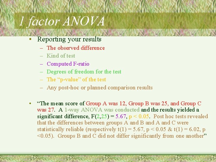
1 factor ANOVA • Reporting your results – – – The observed difference Kind of test Computed F-ratio Degrees of freedom for the test The “p-value” of the test Any post-hoc or planned comparison results • “The mean score of Group A was 12, Group B was 25, and Group C was 27. A 1 -way ANOVA was conducted and the results yielded a significant difference, F(2, 25) = 5. 67, p < 0. 05. Post hoc tests revealed that the differences between groups A and B and A and C were statistically reliable (respectively t(1) = 5. 67, p < 0. 05 & t(1) = 6. 02, p <0. 05). Groups B and C did not differ significantly from one another”

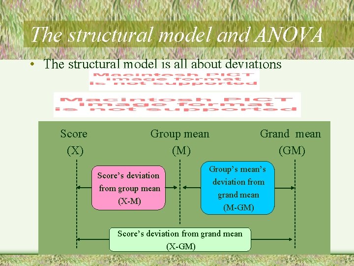
The structural model and ANOVA • The structural model is all about deviations Score (X) Group mean (M) Score’s deviation from group mean (X-M) Grand mean (GM) Group’s mean’s deviation from grand mean (M-GM) Score’s deviation from grand mean (X-GM)

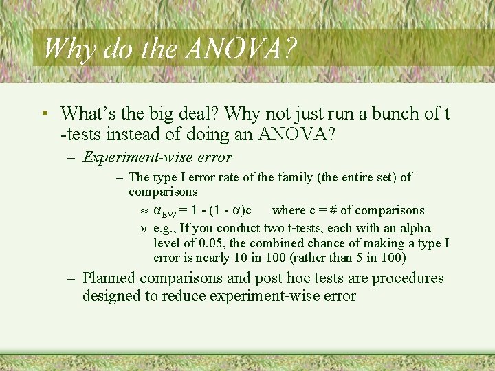
Why do the ANOVA? • What’s the big deal? Why not just run a bunch of t -tests instead of doing an ANOVA? – Experiment-wise error – The type I error rate of the family (the entire set) of comparisons » EW = 1 - (1 - )c where c = # of comparisons » e. g. , If you conduct two t-tests, each with an alpha level of 0. 05, the combined chance of making a type I error is nearly 10 in 100 (rather than 5 in 100) – Planned comparisons and post hoc tests are procedures designed to reduce experiment-wise error

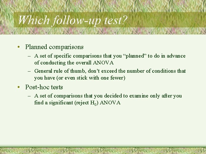
Which follow-up test? • Planned comparisons – A set of specific comparisons that you “planned” to do in advance of conducting the overall ANOVA – General rule of thumb, don’t exceed the number of conditions that you have (or even stick with one fewer) • Post-hoc tests – A set of comparisons that you decided to examine only after you find a significant (reject H 0) ANOVA

Planned Comparisons • Different types – Simple comparisons - testing two groups – Complex comparisons - testing combined groups – Bonferroni procedure • Use more stringent significance level for each comparison • Basic procedure: – Within-groups population variance estimate (denominator) – Between-groups population variance estimate of the two groups of interest (numerator) – Figure F in usual way

Post-hoc tests • Generally, you are testing all of the possible comparisons (rather than just a specific few) – Different types • Tukey’s HSD test • Scheffe test • Others (Fisher’s LSD, Neuman-Keuls test, Duncan test) – Generally they differ with respect to how conservative they are.

Planned Comparisons & Post-Hoc Tests as Contrasts • A contrast is basically a way of assigning numeric values to your grouping variable in a manner that allows you to test a specific difference between two means (or between one mean and a weighted average of two or more other means). • Discuss numbers • Discuss “orthogonal” contrasts

Fixed vs. Random Factors in ANOVA • One-way ANOVAs can use grouping variables that are fixed or random. – Fixed: All levels of the variable of interest are represented by the variable (e. g. , treatment and control, male and female). – Random: The grouping variable represents a random selection of levels of that variable, sampled from a population of levels (e. g. , observers). – For one-way ANOVA, the math is the same either way, but the logic of the test is a little different. (Testing either that means are equal or that the between group variance is 0)

Effect sizes in ANOVA • The effect size for ANOVA is r 2 – Sometimes called 2 (“eta squared”) – The percent of the variance in the dependent variable that is accounted for by the independent variable – Size of effect depends, in part, on degrees of freedom

ANOVA in SPSS • Let’s see how to do a between groups 1 -factor ANOVA in SPSS (and the other tests too)

Within groups (repeated measures) ANOVA • Basics of within groups ANOVA – Repeated measures – Matched samples • Computations • Within groups ANOVA in SPSS

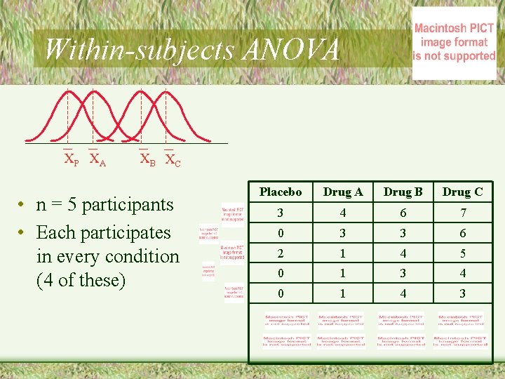
Example • Suppose that you want to compare three brand name pain relievers. – Give each person a drug, wait 15 minutes, then ask them to keep their hand in a bucket of cold water as long as they can. The next day, repeat (with a different drug) • Dependent variable: time in ice water • Independent variable: 4 levels, within groups – – Placebo Drug A Drug B Drug C

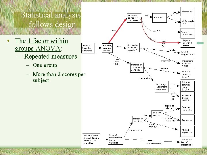
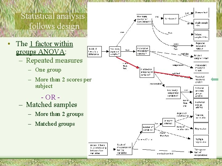
Statistical analysis follows design • The 1 factor within groups ANOVA: – Repeated measures – One group – More than 2 scores per subject

Statistical analysis follows design • The 1 factor within groups ANOVA: – Repeated measures – One group – More than 2 scores per subject - OR – Matched samples – More than 2 groups – Matched groups

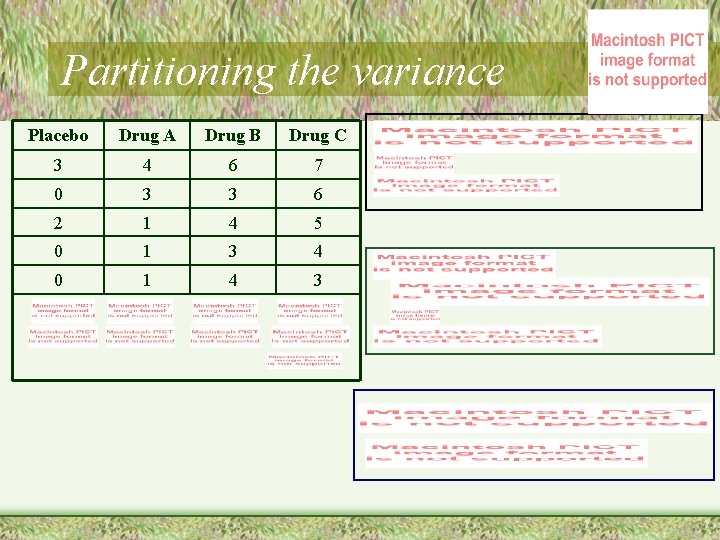
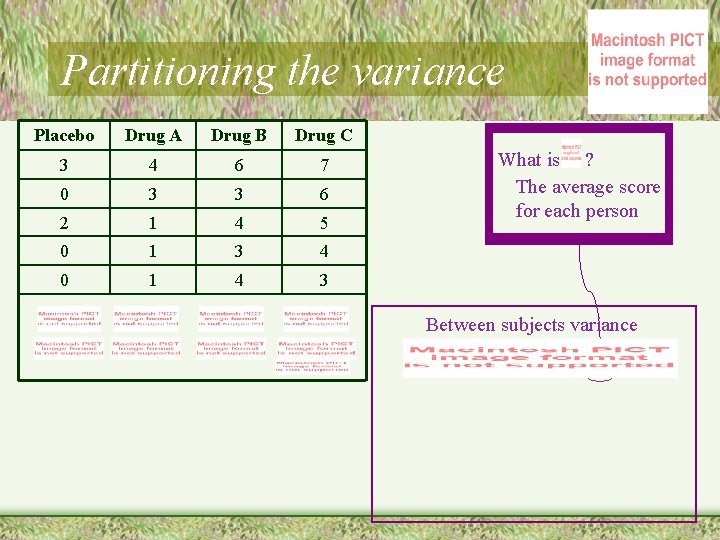
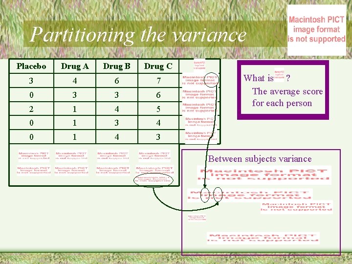
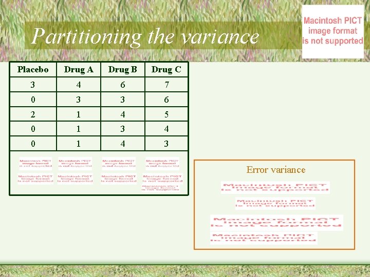
Within-subjects ANOVA XP XA XB XC • n = 5 participants • Each participates in every condition (4 of these) Placebo Drug A Drug B Drug C 3 4 6 7 0 3 3 6 2 1 4 5 0 1 3 4 0 1 4 3

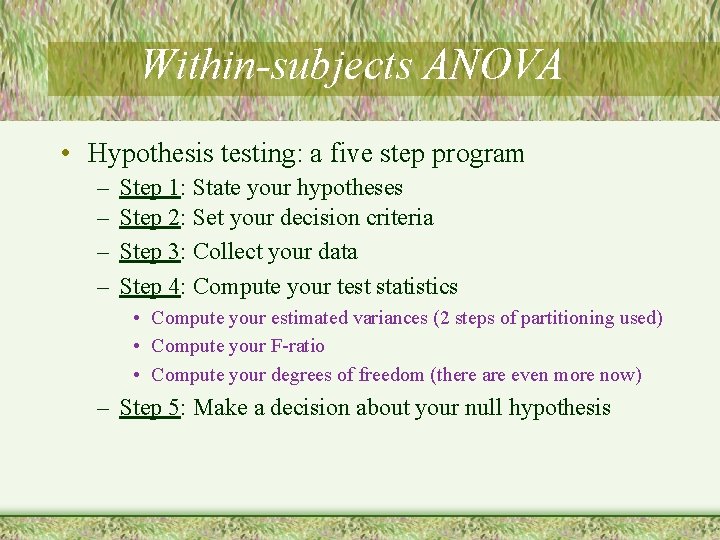
Within-subjects ANOVA • Hypothesis testing: a five step program – – Step 1: State your hypotheses Step 2: Set your decision criteria Step 3: Collect your data Step 4: Compute your test statistics • Compute your estimated variances (2 steps of partitioning used) • Compute your F-ratio • Compute your degrees of freedom (there are even more now) – Step 5: Make a decision about your null hypothesis

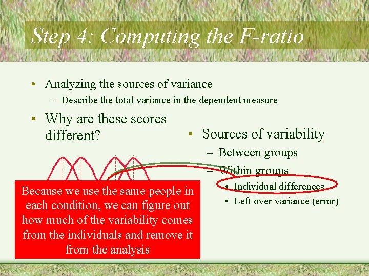
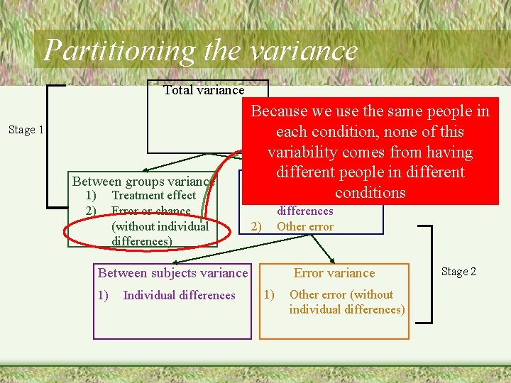
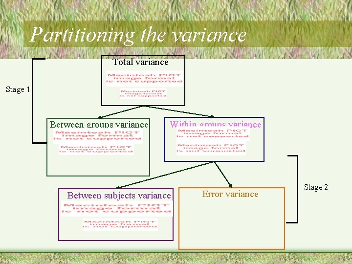
Step 4: Computing the F-ratio • Analyzing the sources of variance – Describe the total variance in the dependent measure • Why are these scores different? • Sources of variability – Between groups – Within groups Because we use the same people in each condition, figure out XP XA we. Xcan B XC how much of the variability comes from the individuals and remove it from the analysis • Individual differences • Left over variance (error)

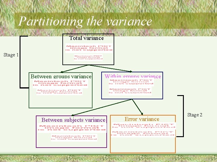
Partitioning the variance Total variance Stage 1 Between groups variance Within groups variance

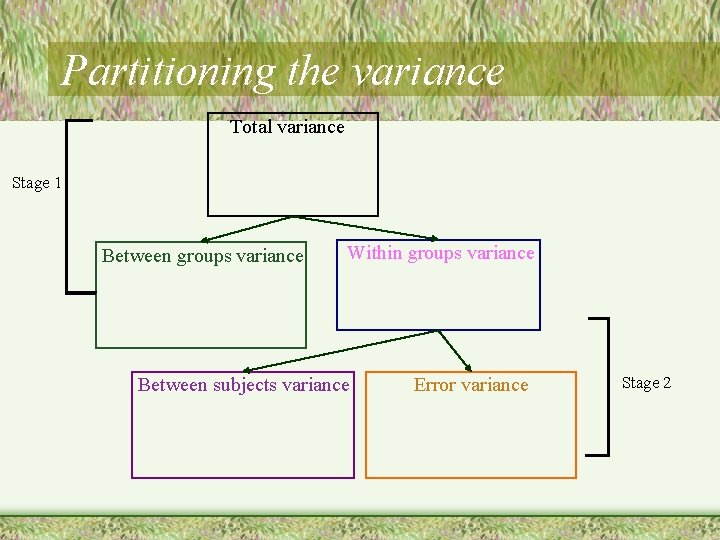
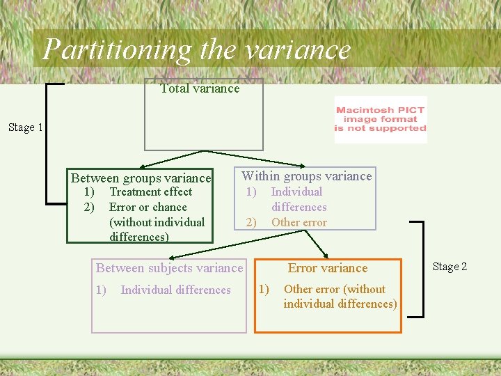
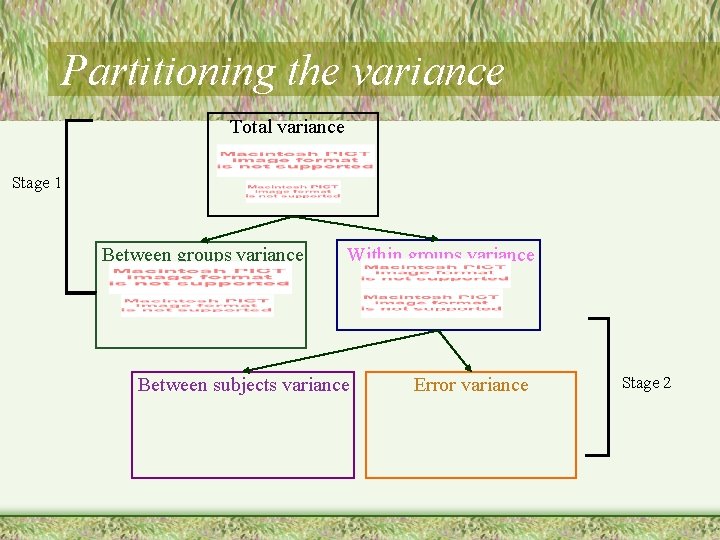
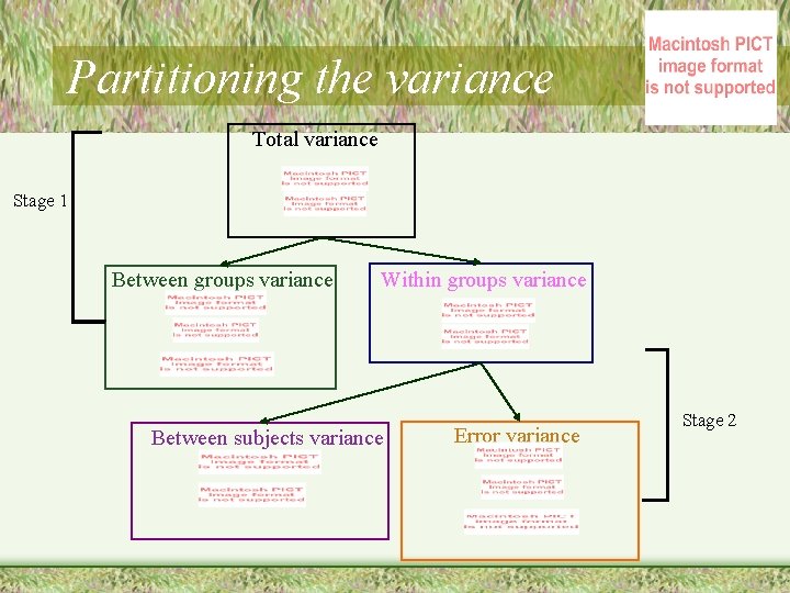
Partitioning the variance Total variance Stage 1 Between groups variance Within groups variance Between subjects variance Error variance Stage 2

Partitioning the variance Total variance Stage 1 Between groups variance 1) 2) Treatment effect Error or chance (without individual differences) Because we use the same people in each condition, none of this variability comes from having different people in different Within groups variance 1) Individual conditions differences Other error 2) Between subjects variance 1) Individual differences Error variance 1) Other error (without individual differences) Stage 2

Step 4: Computing the F-ratio • The F ratio – Ratio of the between-groups variance estimate to the population error variance estimate F-ratio = Observed variance Variance from chance

Partitioning the variance Total variance Stage 1 Between groups variance 1) 2) Within groups variance Treatment effect Error or chance (without individual differences) 1) Individual differences Other error 2) Between subjects variance 1) Individual differences Error variance 1) Other error (without individual differences) Stage 2

Partitioning the variance Total variance Stage 1 Between groups variance Within groups variance

Partitioning the variance Placebo Drug A Drug B Drug C 3 4 6 7 0 3 3 6 2 1 4 5 0 1 3 4 0 1 4 3

Partitioning the variance Total variance Stage 1 Between groups variance Within groups variance Between subjects variance Error variance Stage 2

Partitioning the variance Placebo Drug A Drug B Drug C 3 4 6 7 0 3 3 6 2 1 4 5 0 1 3 4 0 1 4 3 What is ? The average score for each person Between subjects variance

Partitioning the variance Placebo Drug A Drug B Drug C 3 4 6 7 0 3 3 6 2 1 4 5 0 1 3 4 0 1 4 3 What is ? The average score for each person Between subjects variance

Partitioning the variance Total variance Stage 1 Between groups variance Within groups variance Between subjects variance Error variance Stage 2

Partitioning the variance Placebo Drug A Drug B Drug C 3 4 6 7 0 3 3 6 2 1 4 5 0 1 3 4 0 1 4 3 Error variance

Partitioning the variance Total variance Stage 1 Between groups variance Within groups variance Between subjects variance Error variance Stage 2

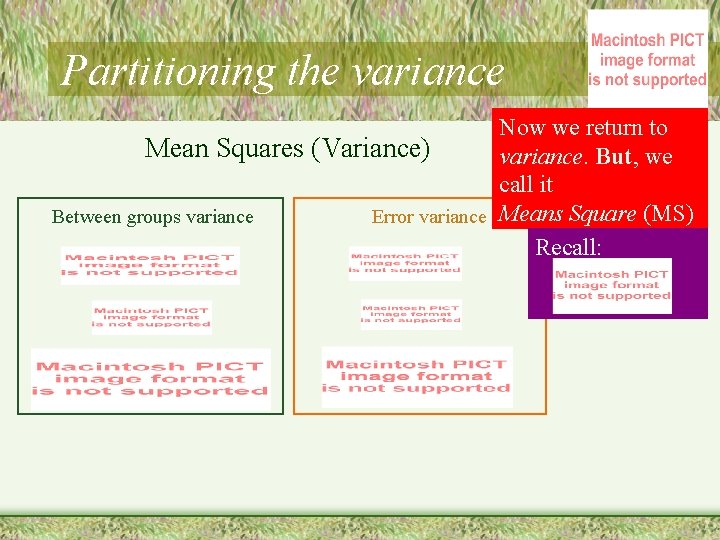
Partitioning the variance Now we return to Mean Squares (Variance) variance. But, we call it Between groups variance Error variance Means Square (MS) Recall:

Partitioning the variance Total variance Stage 1 Between groups variance Within groups variance Between subjects variance Error variance Stage 2

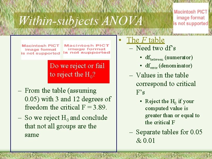
Within-subjects ANOVA • The F table – Need two df’s Do we reject or fail to reject the H 0? – From the table (assuming 0. 05) with 3 and 12 degrees of freedom the critical F = 3. 89. – So we reject H 0 and conclude that not all groups are the same • dfbetween (numerator) • dferror (denominator) – Values in the table correspond to critical F’s • Reject the H 0 if your computed value is greater than or equal to the critical F – Separate tables for 0. 05 & 0. 01

Within-subjects ANOVA in SPSS – Setting up the file – Running the analysis – Looking at the output

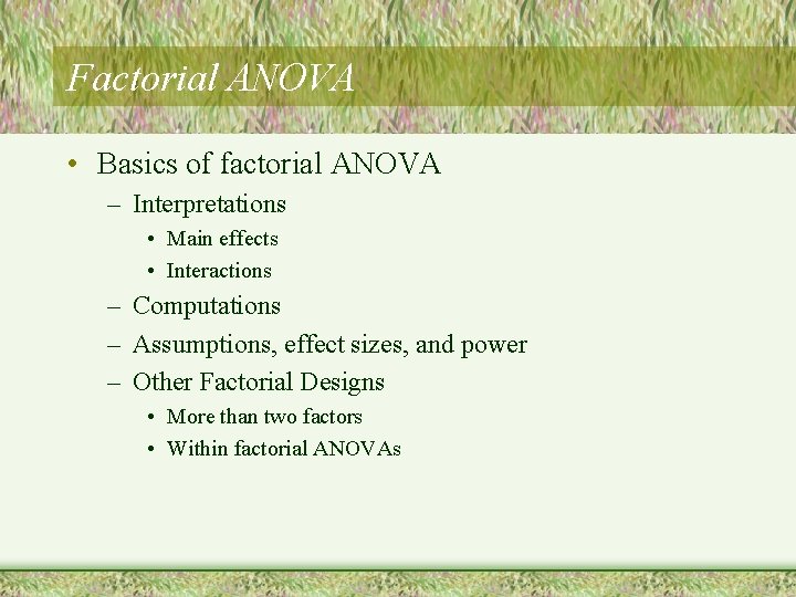
Factorial ANOVA • Basics of factorial ANOVA – Interpretations • Main effects • Interactions – Computations – Assumptions, effect sizes, and power – Other Factorial Designs • More than two factors • Within factorial ANOVAs

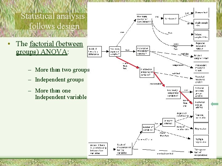
Statistical analysis follows design • The factorial (between groups) ANOVA: – More than two groups – Independent groups – More than one Independent variable

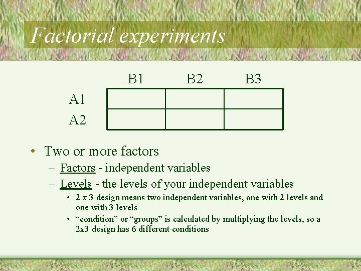
Factorial experiments B 1 B 2 B 3 A 1 A 2 • Two or more factors – Factors - independent variables – Levels - the levels of your independent variables • 2 x 3 design means two independent variables, one with 2 levels and one with 3 levels • “condition” or “groups” is calculated by multiplying the levels, so a 2 x 3 design has 6 different conditions

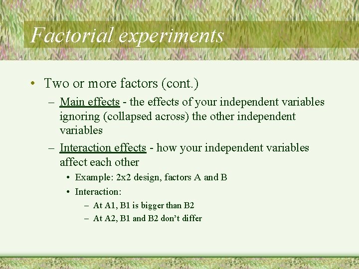
Factorial experiments • Two or more factors (cont. ) – Main effects - the effects of your independent variables ignoring (collapsed across) the other independent variables – Interaction effects - how your independent variables affect each other • Example: 2 x 2 design, factors A and B • Interaction: – At A 1, B 1 is bigger than B 2 – At A 2, B 1 and B 2 don’t differ

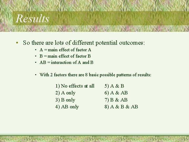
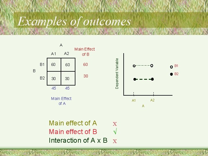
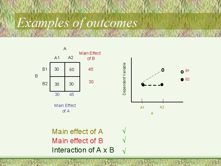
Results • So there are lots of different potential outcomes: • A = main effect of factor A • B = main effect of factor B • AB = interaction of A and B • With 2 factors there are 8 basic possible patterns of results: 1) No effects at all 2) A only 3) B only 4) AB only 5) A & B 6) A & AB 7) B & AB 8) A & B & AB

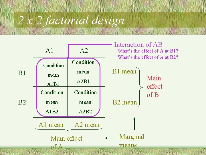
2 x 2 factorial design A 1 Condition B 1 mean A 1 B 1 B 2 A 2 Condition mean Interaction of AB What’s the effect of A at B 1? What’s the effect of A at B 2? B 1 mean A 2 B 1 Condition mean A 1 B 2 A 2 B 2 A 1 mean A 2 mean Main effect of A B 2 mean Marginal means Main effect of B

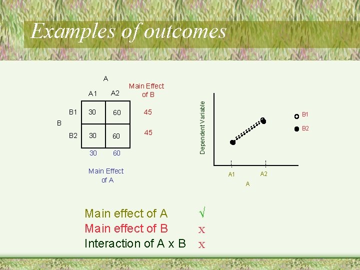
A B 1 A 2 Main Effect of B 30 60 45 30 60 B B 2 Dependent Variable Examples of outcomes Main Effect of A Main effect of B Interaction of A x B B 1 B 2 A 1 A √ X X

A B 1 A 2 Main Effect of B 60 60 60 B B 2 30 30 45 45 30 Dependent Variable Examples of outcomes Main Effect of A Main effect of A X Main effect of B √ Interaction of A x B X B 1 B 2 A 1 A

A B 1 A 2 Main Effect of B 60 30 45 30 60 45 45 45 B B 2 Dependent Variable Examples of outcomes Main Effect of A Main effect of A X Main effect of B X Interaction of A x B √ B 1 B 2 A 1 A

A B 1 A 2 Main Effect of B 30 60 45 30 30 45 B B 2 Dependent Variable Examples of outcomes Main Effect of A Main effect of B Interaction of A x B B 1 B 2 A 1 A √ √ √

Factorial Designs • Benefits of factorial ANOVA (over doing separate 1 way ANOVA experiments) – Interaction effects – One should always consider the interaction effects before trying to interpret the main effects – Adding factors decreases the variability – Because you’re controlling more of the variables that influence the dependent variable – This increases the statistical Power of the statistical tests

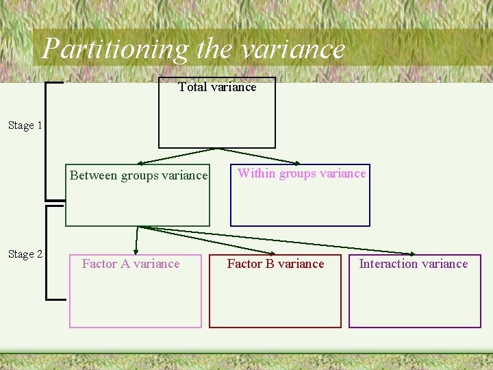
Basic Logic of the Two-Way ANOVA • Same basic math as we used before, but now there additional ways to partition the variance • The three F ratios – Main effect of Factor A (rows) – Main effect of Factor B (columns) – Interaction effect of Factors A and B

Partitioning the variance Total variance Stage 1 Between groups variance Stage 2 Factor A variance Within groups variance Factor B variance Interaction variance

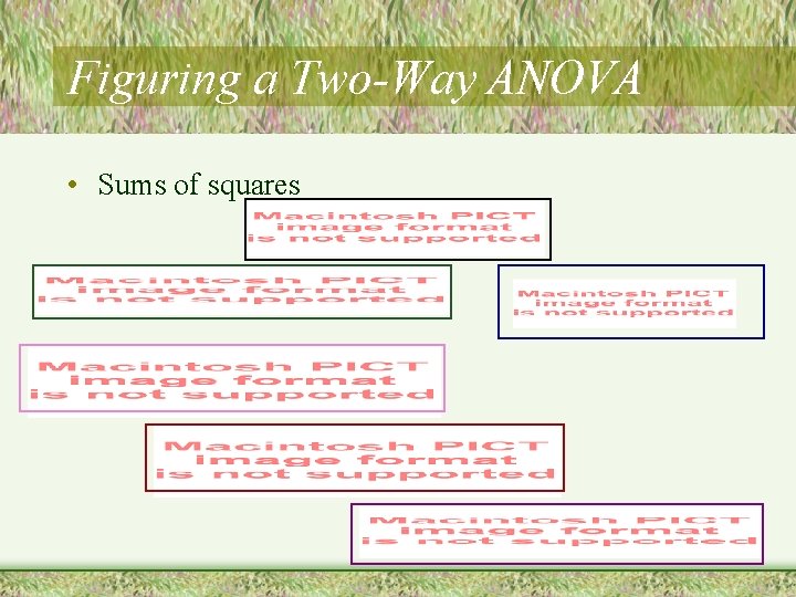
Figuring a Two-Way ANOVA • Sums of squares

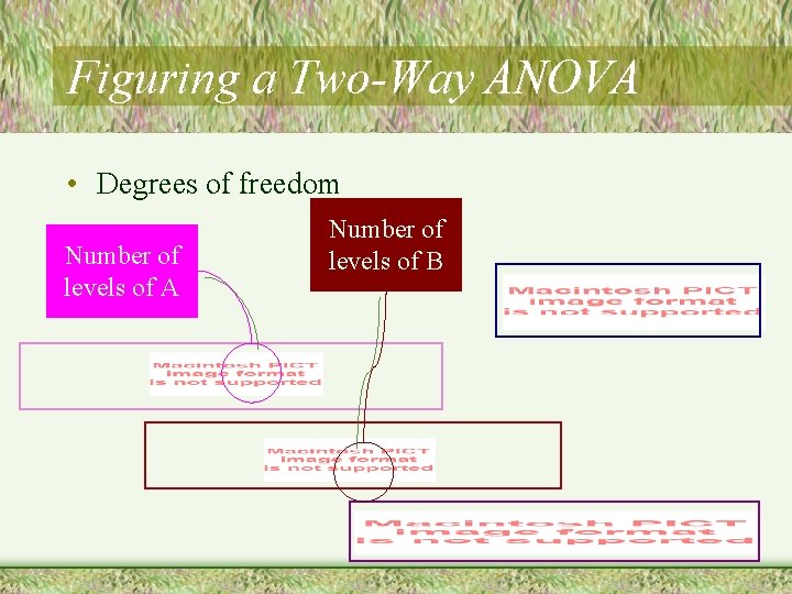
Figuring a Two-Way ANOVA • Degrees of freedom Number of levels of A Number of levels of B

Figuring a Two-Way ANOVA • Means squares (estimated variances)

Figuring a Two-Way ANOVA • F-ratios

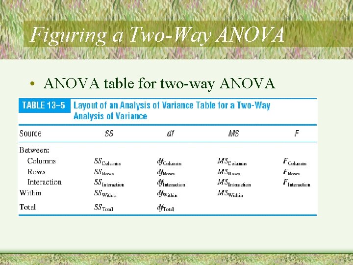
Figuring a Two-Way ANOVA • ANOVA table for two-way ANOVA

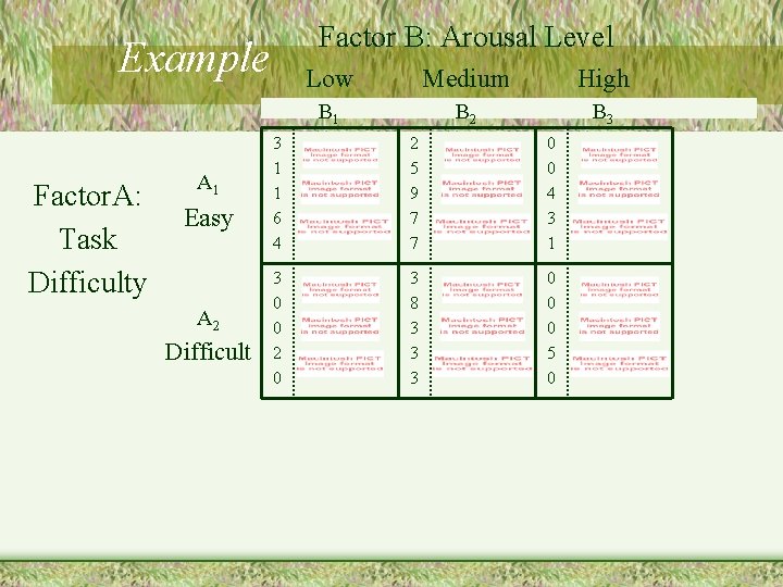
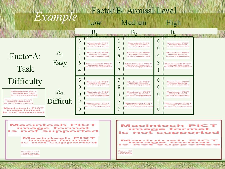
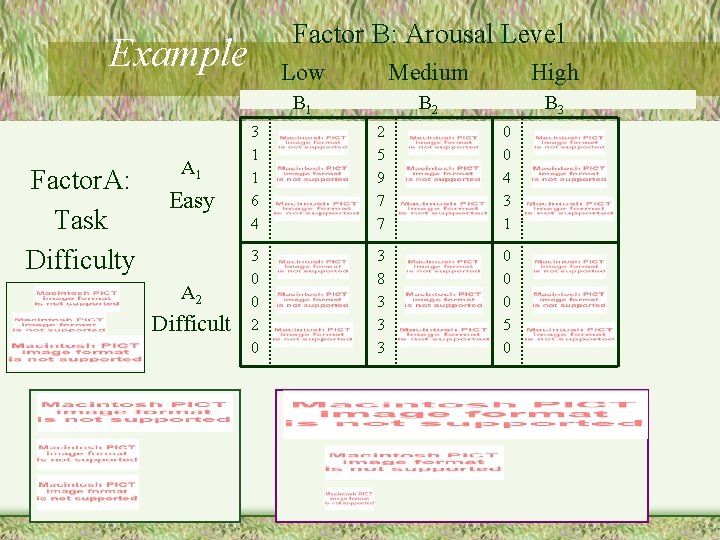
Factor B: Arousal Level Example Factor. A: Task Difficulty A 1 Easy A 2 Difficult Low Medium High B 1 B 2 B 3 3 1 1 6 4 2 5 9 7 7 0 0 4 3 1 3 0 0 2 0 3 8 3 3 3 0 0 0 5 0

Factor B: Arousal Level Example Factor. A: Task Difficulty A 1 Easy A 2 Difficult Low Medium High B 1 B 2 B 3 3 1 1 6 4 2 5 9 7 7 0 0 4 3 1 3 0 0 2 0 3 8 3 3 3 0 0 0 5 0

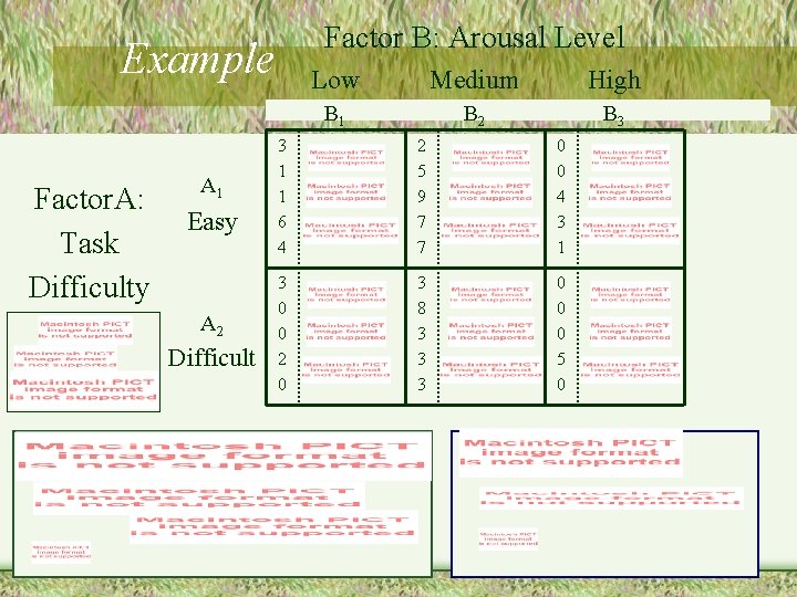
Factor B: Arousal Level Example Factor. A: Task Difficulty A 1 Easy A 2 Difficult Low Medium High B 1 B 2 B 3 3 1 1 6 4 2 5 9 7 7 0 0 4 3 1 3 0 0 2 0 3 8 3 3 3 0 0 0 5 0

Factor B: Arousal Level Example Factor. A: Task Difficulty A 1 Easy A 2 Difficult Low Medium High B 1 B 2 B 3 3 1 1 6 4 2 5 9 7 7 0 0 4 3 1 3 0 0 2 0 3 8 3 3 3 0 0 0 5 0

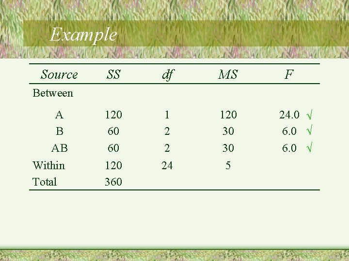
Example Source SS df MS A B AB 120 60 60 1 2 2 120 30 30 Within Total 120 360 24 5 F Between 24. 0 √ 6. 0 √

Assumptions in Two-Way ANOVA • Populations follow a normal curve • Populations have equal variances • Assumptions apply to the populations that go with each cell

Effect Size in Factorial ANOVA

Extensions & Special Cases of Factorial ANOVA • Three-way and higher ANOVA designs • Repeated measures ANOVA • Mixed factorial ANOCA

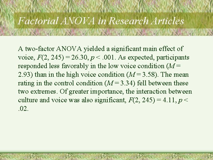
Factorial ANOVA in Research Articles A two-factor ANOVA yielded a significant main effect of voice, F(2, 245) = 26. 30, p <. 001. As expected, participants responded less favorably in the low voice condition (M = 2. 93) than in the high voice condition (M = 3. 58). The mean rating in the control condition (M = 3. 34) fell between these two extremes. Of greater importance, the interaction between culture and voice was also significant, F(2, 245) = 4. 11, p <. 02.

Repeated Measures & Mixed Factorial ANOVA • Basics of repeated measures factorial ANOVA – Using SPSS • Basics of mixed factorial ANOVA – Using SPSS • Similar to the between groups factorial ANOVA – Main effects and interactions – Multiple sources for the error terms (different denominators for each main effect)

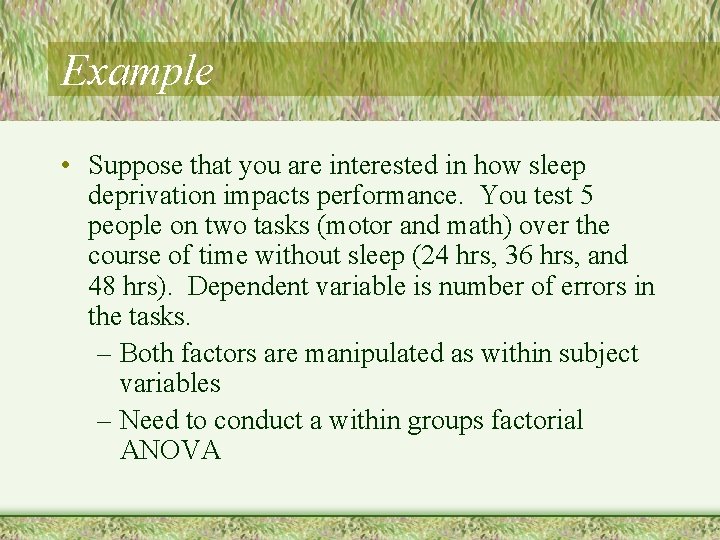
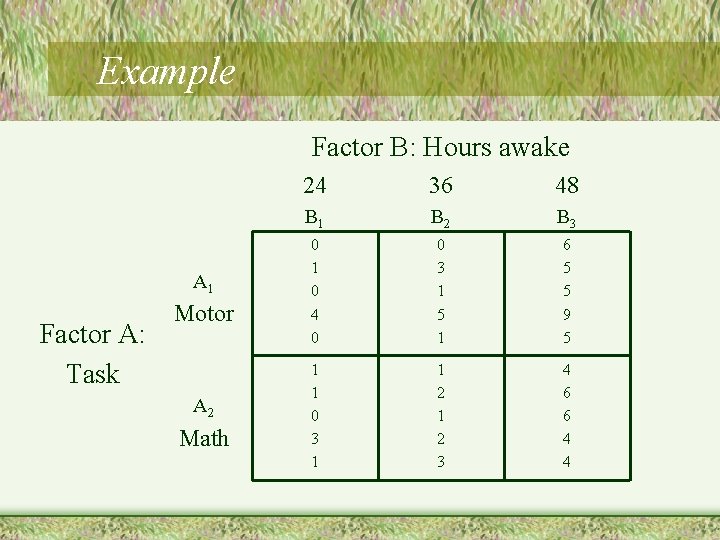
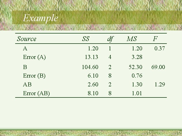
Example • Suppose that you are interested in how sleep deprivation impacts performance. You test 5 people on two tasks (motor and math) over the course of time without sleep (24 hrs, 36 hrs, and 48 hrs). Dependent variable is number of errors in the tasks. – Both factors are manipulated as within subject variables – Need to conduct a within groups factorial ANOVA

Example Factor B: Hours awake A 1 Factor A: Task Motor A 2 Math 24 36 48 B 1 B 2 B 3 0 1 0 4 0 0 3 1 5 1 6 5 5 9 5 1 1 0 3 1 1 2 3 4 6 6 4 4

Example Source A Error (A) B Error (B) AB Error (AB) SS df MS F 1. 20 13. 13 1 4 1. 20 3. 28 0. 37 104. 60 6. 10 2. 60 8. 10 2 8 52. 30 0. 76 1. 30 1. 01 69. 00 1. 29

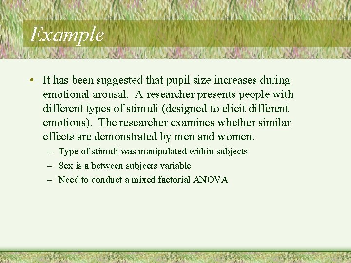
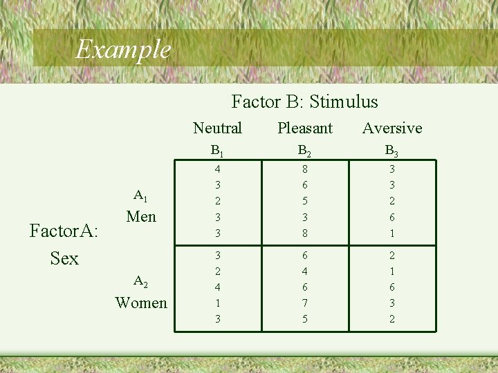
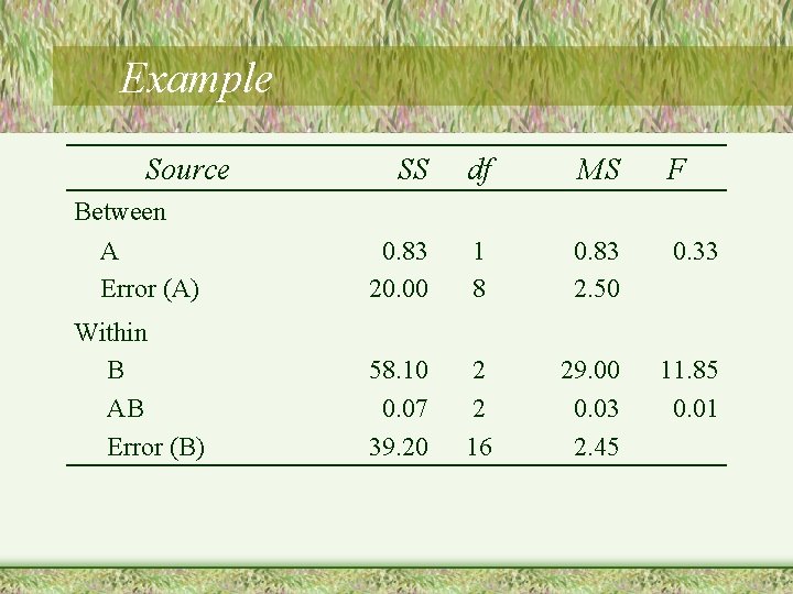
Example • It has been suggested that pupil size increases during emotional arousal. A researcher presents people with different types of stimuli (designed to elicit different emotions). The researcher examines whether similar effects are demonstrated by men and women. – Type of stimuli was manipulated within subjects – Sex is a between subjects variable – Need to conduct a mixed factorial ANOVA

Example Factor B: Stimulus A 1 Factor. A: Sex Men A 2 Women Neutral Pleasant Aversive B 1 B 2 B 3 4 3 2 3 3 8 6 5 3 8 3 3 2 6 1 3 2 4 1 3 6 4 6 7 5 2 1 6 3 2

Example Source SS df MS F Between A Error (A) 0. 83 20. 00 1 8 0. 83 2. 50 0. 33 Within B AB Error (B) 58. 10 0. 07 39. 20 2 2 16 29. 00 0. 03 2. 45 11. 85 0. 01