Anomaly detection in Categorical Datasets Kaustav Das Jeff

Anomaly detection in Categorical Datasets Kaustav Das, Jeff Schneider Machine Learning Department Carnegie Mellon University 1

Outline o o o Problem Motivation/Overview Related Work Conditional Anomaly Marginal Anomaly Datasets and Results 2

Problem Motivation o Detect anomalous records in large amount of record based data Import of Containers Astronomical Data Network Intrusion Detection Emergency Department 3

Problem Overview Training Data: o Categorical dataset – categorize real values. o Large number of records – 100, 000 to 1 million. o Unlabelled: A small fraction of them (<1 -2%) can be anomalous. o Attributes can have high arity of up to 5000 -10, 000. Test Data: o Same properties as above. o Can have any fraction of anomalous records. Goal: o To detect records in the test set that are ‘anomalous’. o More generally, score each test record with the degree of anomalousness. o Flag records based on the desired false positive rate. 4

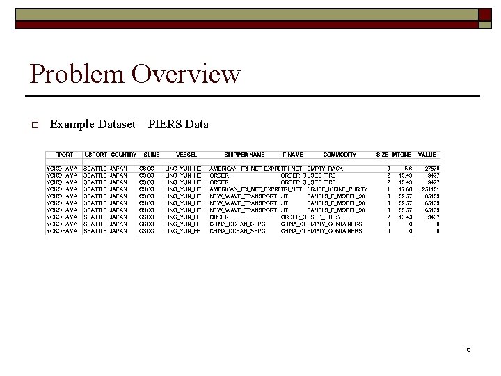
Problem Overview o Example Dataset – PIERS Data 5

Related Work o Likelihood Based Methods n n Dependency Trees [Pelleg ’ 04] Bayes Network o o o Network Intrusion Detection [Ye and Xu ’ 00; Bronstein et al. ’ 01] Malicious Email Detection [Shih et al. ’ 04] Disease Outbreak Detection [Wong et al. ’ 03] q Learn a probability distribution model from training data. q Anomalies: Test set records having unusually low likelihood in the learnt model. 6

Related Work o Likelihood Based Methods n n Dependency Trees [Pelleg ’ 04] Bayes Network o o Network Intrusion Detection [Ye and Xu ’ 00; Bronstein et al. ’ 01] Malicious Email Detection [Shih et al. ’ 04] Disease Outbreak Detection [Wong et al. ’ 03] Association Rule Learners n LERAD o o n [Chan et al. ’ 06] q Learn a probability distribution model from training data. q Anomalies: Test set records having unusually low likelihood in the learnt model. Learn rules of the form X → Y Anomaly score depends on P(¬Y|X) Hidden Association Rules [Banderas et al. ’ 05] 7

Outline o o o Problem Motivation/Overview Related Work Conditional Anomaly n n o o Motivation/Definition Algorithm for Testing Records Estimating Probability Values Speedup Tricks Marginal Anomaly Datasets and Results 8

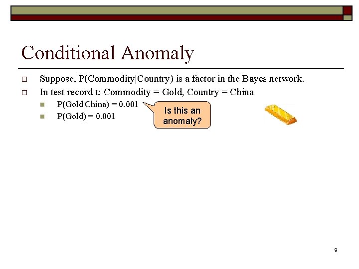
Conditional Anomaly o o Suppose, P(Commodity|Country) is a factor in the Bayes network. In test record t: Commodity = Gold, Country = China n n P(Gold|China) = 0. 001 P(Gold) = 0. 001 Is this an anomaly? 9

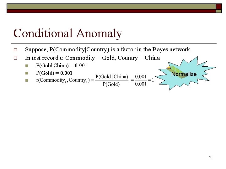
Conditional Anomaly o o Suppose, P(Commodity|Country) is a factor in the Bayes network. In test record t: Commodity = Gold, Country = China n n P(Gold|China) = 0. 001 P(Gold) = 0. 001 Normalize n 10

Conditional Anomaly o o Suppose, P(Commodity|Country) is a factor in the Bayes network. In test record t: Commodity = Gold, Country = China n n P(Gold|China) = 0. 001 P(Gold) = 0. 001 n o Commodity = Copper, Country = China n n P(Copper|China) = 0. 001 P(Copper) = 0. 1 n 11

Conditional Anomaly o r value is defined over two attribute values at and bt of attributes A and B in test record t. o A small r value denotes that there is a strong negative dependence between the occurrence of values at and bt co-occurring in t and r(at , bt) << 1 t is Anomalous !! o 12

Conditional Anomaly o r value is defined over two attribute values at and bt of attributes A and B in test record t. o A small r value denotes that there is a strong negative dependence between the occurrence of values at and bt co-occurring in t and r(at , bt) << 1 t is Anomalous !! In general, we can consider sets of attributes A and B to calculate r. For example, o o o We limit the number of attributes in each set to k. Hence, we consider up to 2 k attributes at a time. 13

Conditional Anomaly – Algorithm o Algorithm for testing record t n For each mutually exclusive pair of attribute sets {A, B} compute: Exponential number of r values: O(m 2 k) n Score the record t based on all the r values. o o Heuristic 1: Assign the minimum r value as the score Heuristic 2 (Combining evidence) : Combine evidence from other subsets of attributes by taking product of r values. 14

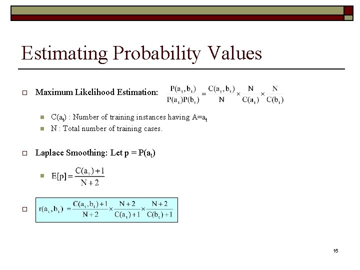
Estimating Probability Values o Maximum Likelihood Estimation: n n o C(at) : Number of training instances having A=at N : Total number of training cases. Laplace Smoothing: Let p = P(at) n o 15

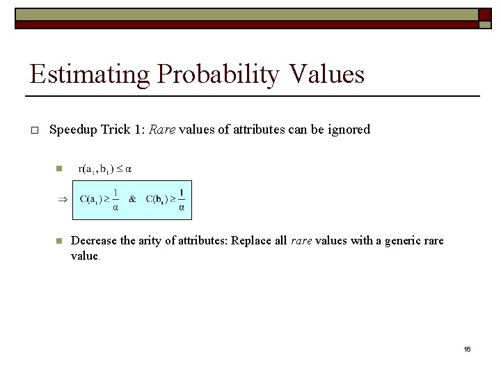
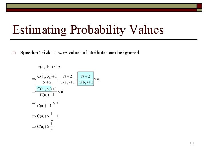
Estimating Probability Values o Speedup Trick 1: Rare values of attributes can be ignored n n Decrease the arity of attributes: Replace all rare values with a generic rare value. 16

Estimating Probability Values o Speedup Trick 2: To estimate counts from the training data, use a very efficient caching data-structure: AD-Tree [Moore and Lee ’ 98] n n n Naïve method is O(N). AD -Tree pre-computes the values of most queries, and requires a small computation for some queries. It is independent of N. Construct an AD-Tree on the reduced arity attributes. 17

Outline o o o Problem Motivation/Overview Related Work Conditional Anomaly Marginal Anomaly Datasets and Results 18

Marginal Anomaly o What about rare values? n n o o Import of Plutonium Import of $1 million worth What is the probability of seeing something this rare or rarer? Consider attribute set A of up to k attributes. 19

Marginal Anomaly What about rare values? n n o What is the probability of seeing something this rare or rarer? Consider attribute set A of up to k attributes. Probability of occurrence o Import of Plutonium Import of $1 million worth Probability of occurrence o a 1 a 2 a 3 a 4 a 5 a 49 a 50 Values of attribute A b 1 b 2 b 3 b 4 b 5 b 6 b 7 b 8 b 9 Values of attribute B 20

Outline o o o Problem Motivation/Overview Related Work Conditional Anomaly Marginal Anomaly Datasets and Results 21

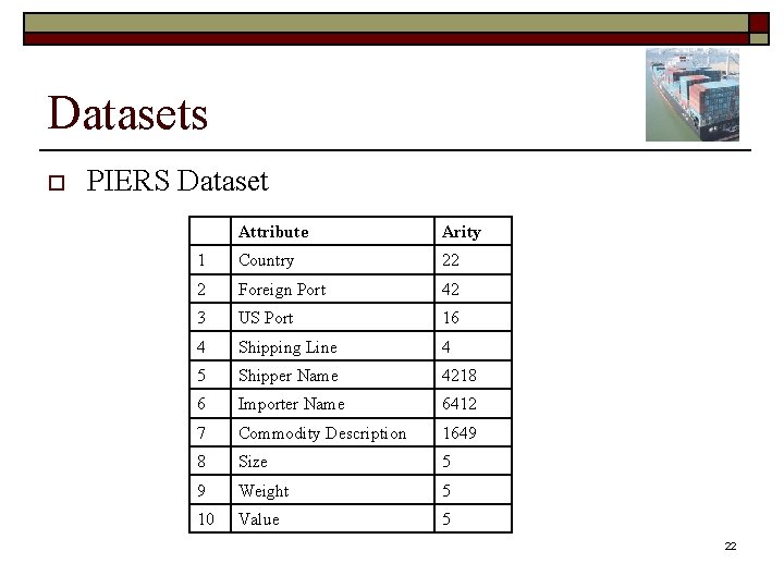
Datasets o PIERS Dataset Attribute Arity 1 Country 22 2 Foreign Port 42 3 US Port 16 4 Shipping Line 4 5 Shipper Name 4218 6 Importer Name 6412 7 Commodity Description 1649 8 Size 5 9 Weight 5 10 Value 5 22

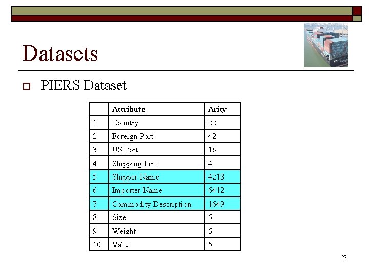
Datasets o PIERS Dataset Attribute Arity 1 Country 22 2 Foreign Port 42 3 US Port 16 4 Shipping Line 4 5 Shipper Name 4218 6 Importer Name 6412 7 Commodity Description 1649 8 Size 5 9 Weight 5 10 Value 5 23

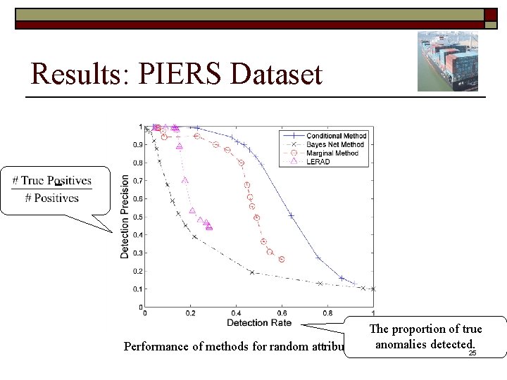
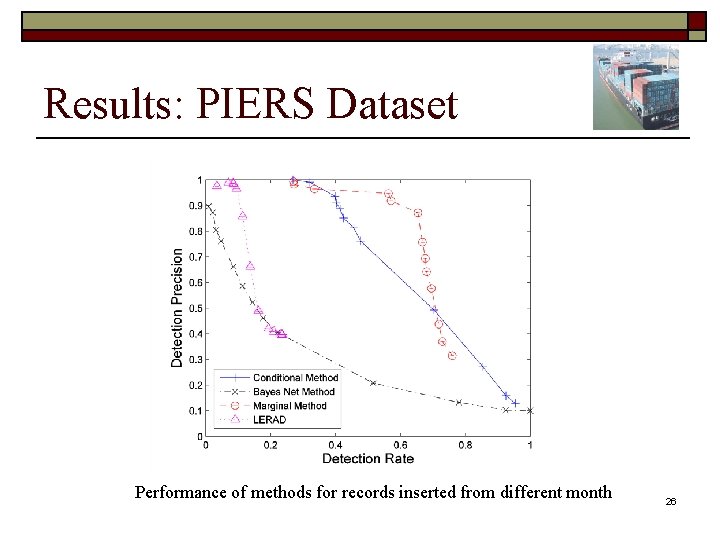
Datasets o PIERS Dataset n n No labeled anomalies. Anomaly Generation – Method 1 o o o n Anomaly Generation – Method 2 o n n Select a test record to be modified. Randomly choose an attribute. Flip the value of the chosen attribute, drawing from the attribute marginal. Insert records from a different time-period. 100, 000 training records and 10, 000 test records. 10% of test record are generated to be anomalous. 24

Results: PIERS Dataset The proportion of true Performance of methods for random attribute flipsanomalies detected. 25

Results: PIERS Dataset Performance of methods for records inserted from different month 26

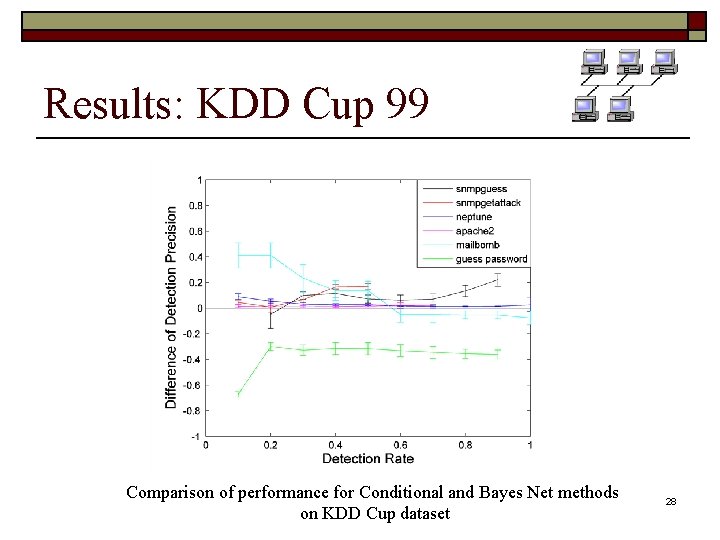
Datasets o KDD Cup 99 Dataset n n Records correspond to individual network sessions. Features: o Basic features of an individual TCP connection: n n n o Features obtained using some domain knowledge: n n o number of connections to the same service, etc. In total there are 41 features, most of them taking continuous values. o n number of file creation operations number of failed login attempts, etc. Features computed using a two second time window: n n duration protocol type number of bytes transferred, etc. Discretized to 5 levels. We selected six different attack types: o apache 2, guess password, mailbomb, neptune, snmpguess and snmpgetattack. 27

Results: KDD Cup 99 Comparison of performance for Conditional and Bayes Net methods on KDD Cup dataset 28

Summary o Detecting anomalies based on learning single probability distribution model and computing whole record likelihoods is problematic: n n n o High arity leads to detecting rare attribute values. The signal in some features gets washed out in the noise of the rest of the features. Anomalies highlight mistakes in model learning. We propose new approaches to solve this: n n Considering all subsets of features up to some size. Define r-values which can indicate anomalies arising out of co-occurrence of high negatively correlated values. Empirical results on real data sets demonstrate improved anomaly detection. The time and memory requirements for our algorithms is comparable to that of the baseline methods. 29

Thank You! Please visit poster board #39 30

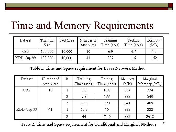
Time and Memory Requirements Dataset Training Size Test Size Number of Attributes Training Time (secs) Testing Time (secs) Memory (MB) CBP 100, 000 10 6. 9 4. 7 4. 5 KDD Cup 99 100, 000 10, 000 41 297 1. 6 152 Table 1: Time and Space requirement for Bayes Network Method Dataset Number of Attributes k Training Time (secs) Testing Time (secs) Memory (MB) Marginal Memory (MB) CBP 10 1 7. 6 16. 8 337 334 2 7. 8 133 338 340 3 9. 3 790 341 489 1 10. 2 15 323 222 2 44 7145 332 2618 KDD Cup 99 41 Table 2: Time and Space requirement for Conditional and Marginal Methods 31

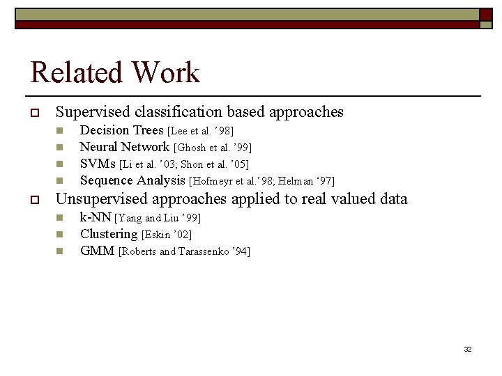
Related Work o Supervised classification based approaches n n o Decision Trees [Lee et al. ’ 98] Neural Network [Ghosh et al. ’ 99] SVMs [Li et al. ’ 03; Shon et al. ’ 05] Sequence Analysis [Hofmeyr et al. ’ 98; Helman ‘ 97] Unsupervised approaches applied to real valued data n n n k-NN [Yang and Liu ’ 99] Clustering [Eskin ’ 02] GMM [Roberts and Tarassenko ’ 94] 32

Estimating Probability Values o Speedup Trick 1: Rare values of attributes can be ignored 33

Marginal Anomaly Detection o o o In test record t, the attribute combination A has value at. Compute C(at), and C(ai) for all values of ai of A which are rarer than at. For each attribute set A, precompute: n n Histogram function, h. A(i) : number of values of A that occur i times in training data. Cumulative histogram, ch. A(i) : number of records having values of A that occur i times or less in the training data. o o o Construct a non-reduced AD-Tree on the training data. 34

Marginal Anomaly Detection o Testing Algorithm for record t n For each composite attribute A compute: n Assign the minimum p-value as the score of record t 35

Grouping o o Group (cluster) the records according to some similarity measure. Find clusters in data with unusual concentration of anomalies. n k-NN n k-means (modes) n GDA (link detection) Define a collection of groups independent of data. Search over all possible groups to find unusual concentration of anomalies n WSARE n Scan Stats 36

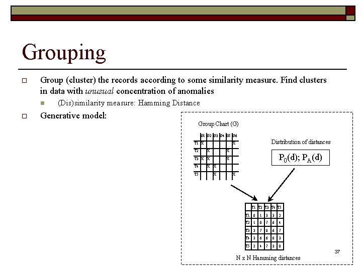
Grouping o Group (cluster) the records according to some similarity measure. Find clusters in data with unusual concentration of anomalies n o (Dis)similarity measure: Hamming Distance Generative model: Group Chart (G) G 1 G 2 G 3 G 4 G 5 G 6 T 1 X T 2 Distribution of distances X X X T 3 X X X T 4 X X T 5 X P 0(d); PA(d) X T 1 T 2 T 3 T 4 T 5 T 1 0 1 3 3 2 T 2 1 0 7 6 4 T 3 3 7 0 6 7 T 4 3 6 6 0 3 T 5 2 4 7 3 0 N x N Hamming distances 37

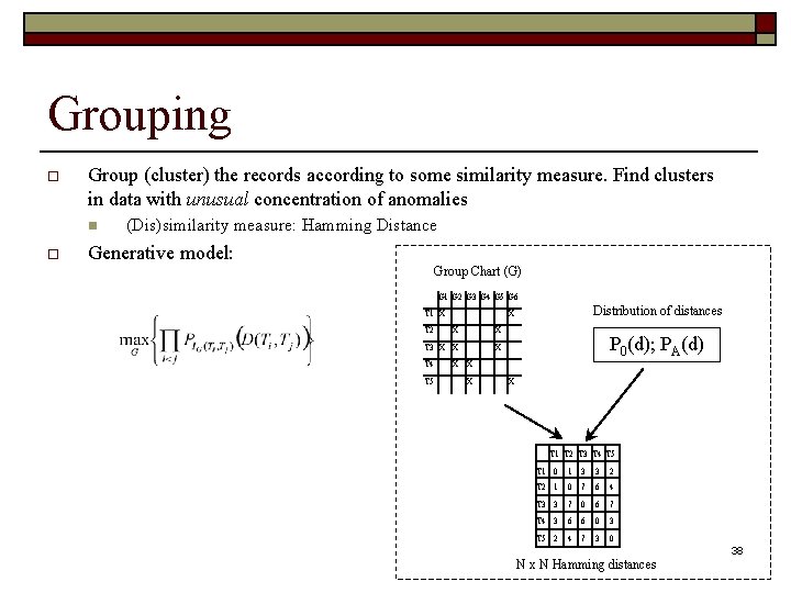
Grouping o Group (cluster) the records according to some similarity measure. Find clusters in data with unusual concentration of anomalies n o (Dis)similarity measure: Hamming Distance Generative model: Group Chart (G) G 1 G 2 G 3 G 4 G 5 G 6 T 1 X T 2 Distribution of distances X X X T 3 X X X T 4 X X T 5 X P 0(d); PA(d) X T 1 T 2 T 3 T 4 T 5 T 1 0 1 3 3 2 T 2 1 0 7 6 4 T 3 3 7 0 6 7 T 4 3 6 6 0 3 T 5 2 4 7 3 0 N x N Hamming distances 38

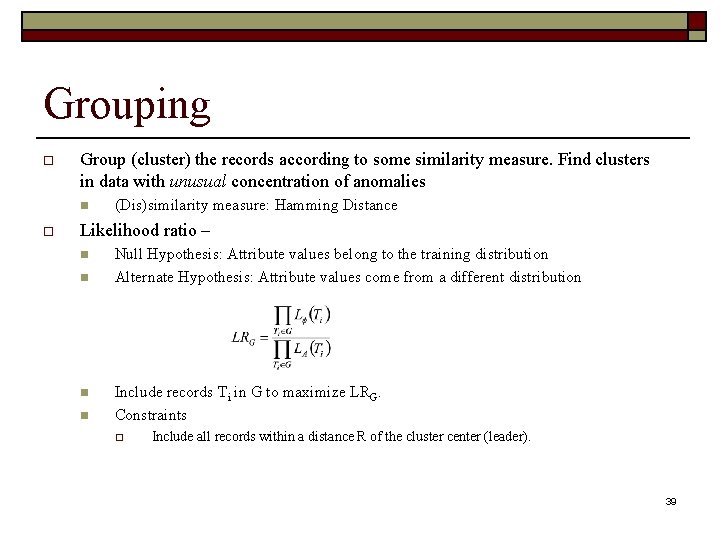
Grouping o Group (cluster) the records according to some similarity measure. Find clusters in data with unusual concentration of anomalies n o (Dis)similarity measure: Hamming Distance Likelihood ratio – n n Null Hypothesis: Attribute values belong to the training distribution Alternate Hypothesis: Attribute values come from a different distribution Include records Ti in G to maximize LRG. Constraints o Include all records within a distance R of the cluster center (leader). 39

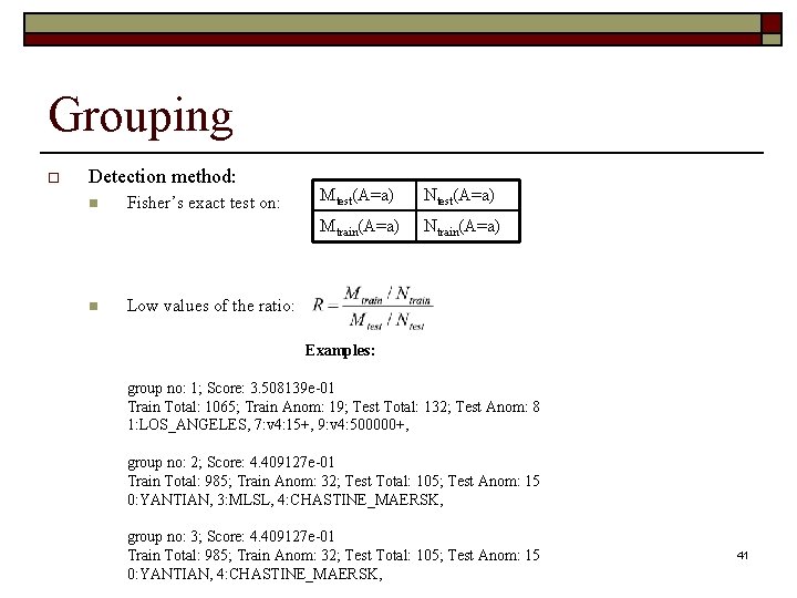
Grouping o o o Define a collection of groups independent of data. Search over all possible groups to find unusual concentration of anomalies All records with matching value(s) of particular attribute(s). Detection method: n n Fisher’s exact test on: Mtest(A=a) Ntest(A=a) Mtrain(A=a) Ntrain(A=a) Low values of the ratio: 40

Grouping o Detection method: n n Fisher’s exact test on: Mtest(A=a) Ntest(A=a) Mtrain(A=a) Ntrain(A=a) Low values of the ratio: Examples: group no: 1; Score: 3. 508139 e-01 Train Total: 1065; Train Anom: 19; Test Total: 132; Test Anom: 8 1: LOS_ANGELES, 7: v 4: 15+, 9: v 4: 500000+, group no: 2; Score: 4. 409127 e-01 Train Total: 985; Train Anom: 32; Test Total: 105; Test Anom: 15 0: YANTIAN, 3: MLSL, 4: CHASTINE_MAERSK, group no: 3; Score: 4. 409127 e-01 Train Total: 985; Train Anom: 32; Test Total: 105; Test Anom: 15 0: YANTIAN, 4: CHASTINE_MAERSK, 41

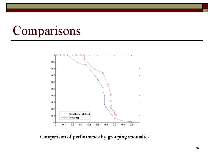
Comparisons Comparison of performance by grouping anomalies 42

Comparisons o o WSARE Mtest(A=a) Ntest(A=a) Ntest(A≠a) Mtrain(A=a) Ntrain(A=a) Ntrain(A≠a) Scan Statistics n Real valued geographic coordinates. 43

Conditional Anomaly o o o A small r value denotes that there is a strong negative dependence between the occurrence of values at and bt. When we observe at and bt co-occurring in a record t and r has an unusually low value, we conclude that this is an anomaly. In general, we can consider sets of attributes A and B to calculate r. For example, We limit the number of attributes in each set to k. Hence, we consider up to 2 k attributes at a time. 44