Announcements Assignments P 0 Python Autograder Tutorial Due

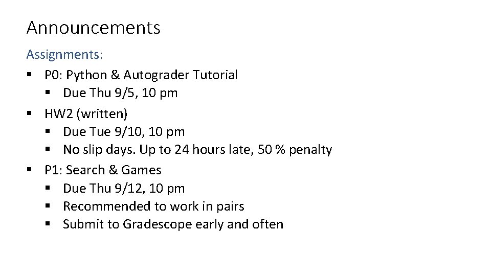
Announcements Assignments: § P 0: Python & Autograder Tutorial § Due Thu 9/5, 10 pm § HW 2 (written) § Due Tue 9/10, 10 pm § No slip days. Up to 24 hours late, 50 % penalty § P 1: Search & Games § Due Thu 9/12, 10 pm § Recommended to work in pairs § Submit to Gradescope early and often

AI: Representation and Problem Solving Adversarial Search Instructors: Pat Virtue & Fei Fang Slide credits: CMU AI, http: //ai. berkeley. edu

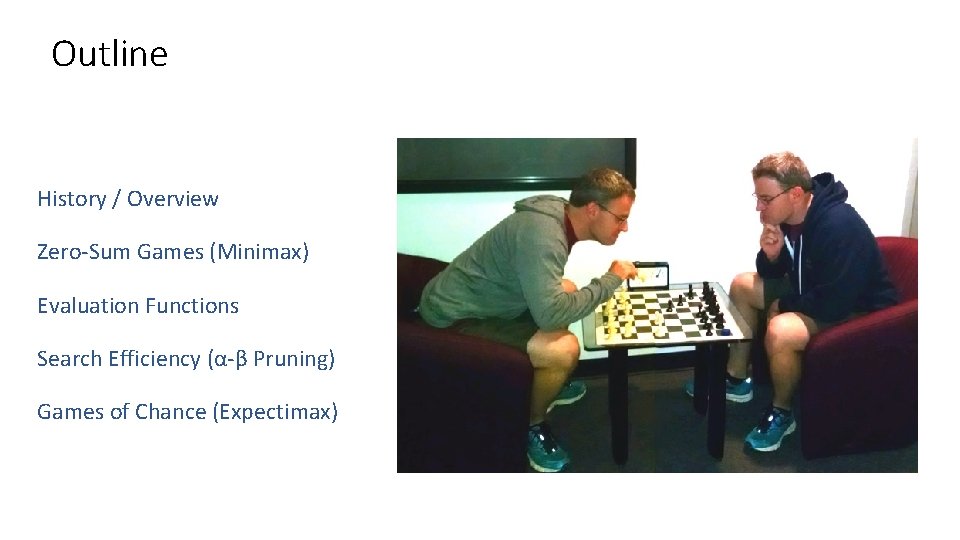
Outline History / Overview Zero-Sum Games (Minimax) Evaluation Functions Search Efficiency (α-β Pruning) Games of Chance (Expectimax)

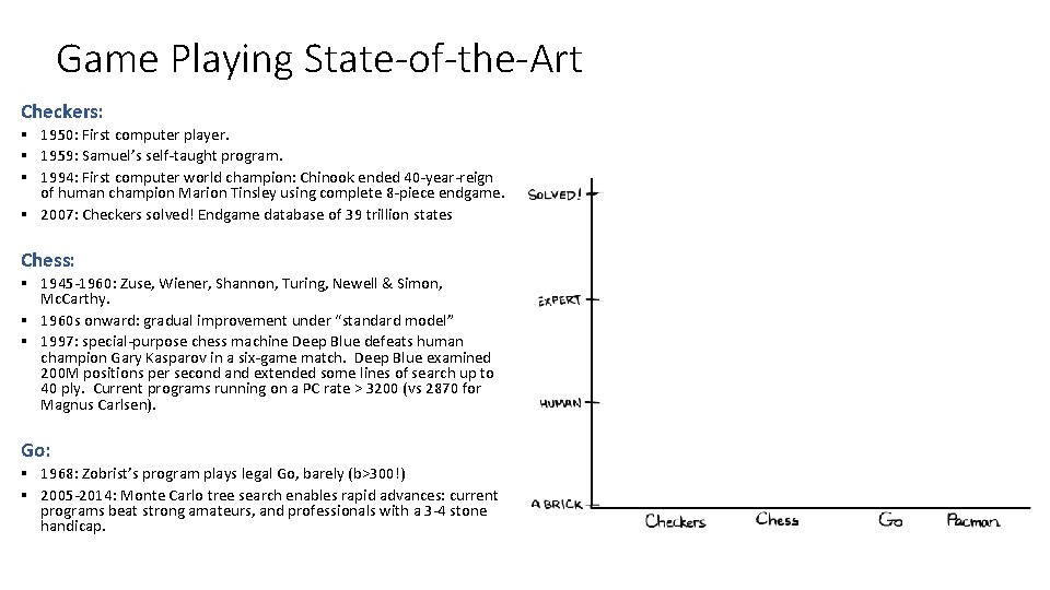
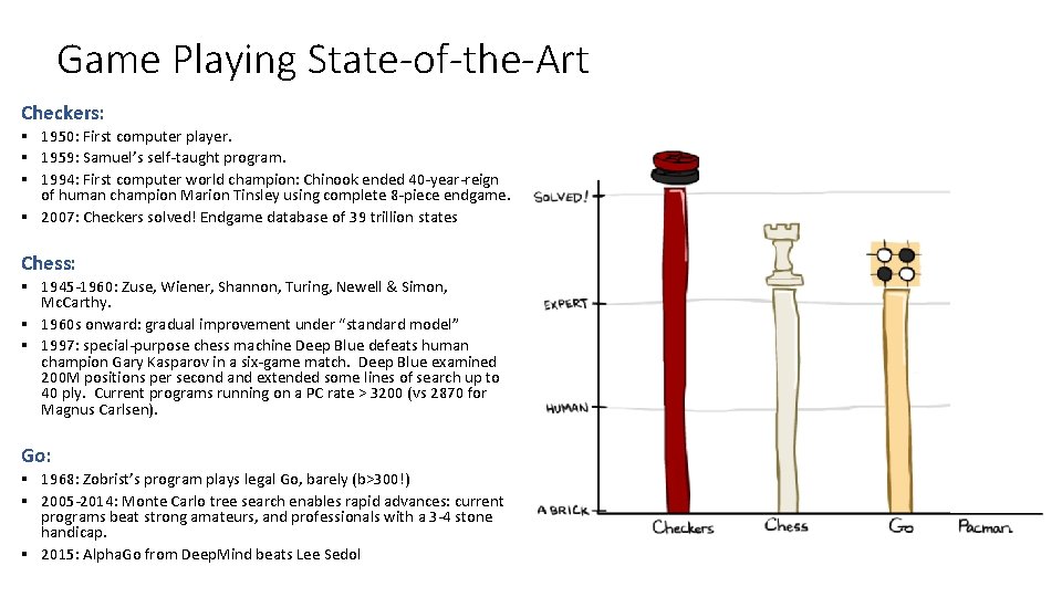
Game Playing State-of-the-Art Checkers: § 1950: First computer player. § 1959: Samuel’s self-taught program. § 1994: First computer world champion: Chinook ended 40 -year-reign of human champion Marion Tinsley using complete 8 -piece endgame. § 2007: Checkers solved! Endgame database of 39 trillion states Chess: § 1945 -1960: Zuse, Wiener, Shannon, Turing, Newell & Simon, Mc. Carthy. § 1960 s onward: gradual improvement under “standard model” § 1997: special-purpose chess machine Deep Blue defeats human champion Gary Kasparov in a six-game match. Deep Blue examined 200 M positions per second and extended some lines of search up to 40 ply. Current programs running on a PC rate > 3200 (vs 2870 for Magnus Carlsen). Go: § 1968: Zobrist’s program plays legal Go, barely (b>300!) § 2005 -2014: Monte Carlo tree search enables rapid advances: current programs beat strong amateurs, and professionals with a 3 -4 stone handicap.

Game Playing State-of-the-Art Checkers: § 1950: First computer player. § 1959: Samuel’s self-taught program. § 1994: First computer world champion: Chinook ended 40 -year-reign of human champion Marion Tinsley using complete 8 -piece endgame. § 2007: Checkers solved! Endgame database of 39 trillion states Chess: § 1945 -1960: Zuse, Wiener, Shannon, Turing, Newell & Simon, Mc. Carthy. § 1960 s onward: gradual improvement under “standard model” § 1997: special-purpose chess machine Deep Blue defeats human champion Gary Kasparov in a six-game match. Deep Blue examined 200 M positions per second and extended some lines of search up to 40 ply. Current programs running on a PC rate > 3200 (vs 2870 for Magnus Carlsen). Go: § 1968: Zobrist’s program plays legal Go, barely (b>300!) § 2005 -2014: Monte Carlo tree search enables rapid advances: current programs beat strong amateurs, and professionals with a 3 -4 stone handicap. § 2015: Alpha. Go from Deep. Mind beats Lee Sedol

Behavior from Computation [Demo: mystery pacman (L 6 D 1)]

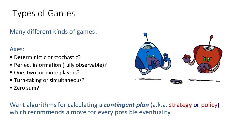
Types of Games Many different kinds of games! Axes: § Deterministic or stochastic? § Perfect information (fully observable)? § One, two, or more players? § Turn-taking or simultaneous? § Zero sum? Want algorithms for calculating a contingent plan (a. k. a. strategy or policy) which recommends a move for every possible eventuality

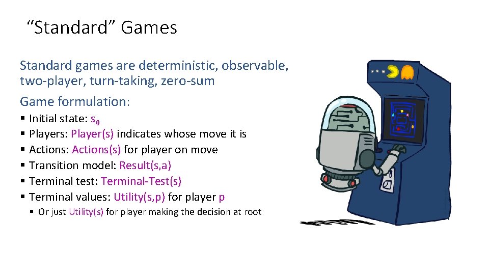
“Standard” Games Standard games are deterministic, observable, two-player, turn-taking, zero-sum Game formulation: § Initial state: s 0 § Players: Player(s) indicates whose move it is § Actions: Actions(s) for player on move § Transition model: Result(s, a) § Terminal test: Terminal-Test(s) § Terminal values: Utility(s, p) for player p § Or just Utility(s) for player making the decision at root

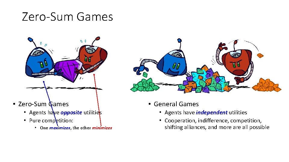
Zero-Sum Games • Zero-Sum Games • Agents have opposite utilities • Pure competition: • One maximizes, the other minimizes • General Games • Agents have independent utilities • Cooperation, indifference, competition, shifting alliances, and more all possible

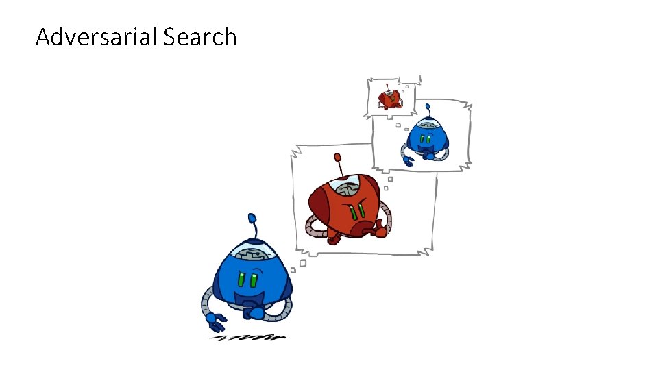
Adversarial Search

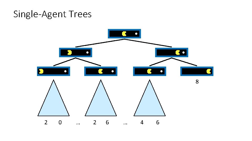
Single-Agent Trees 8 2 0 … 2 6 … 4 6

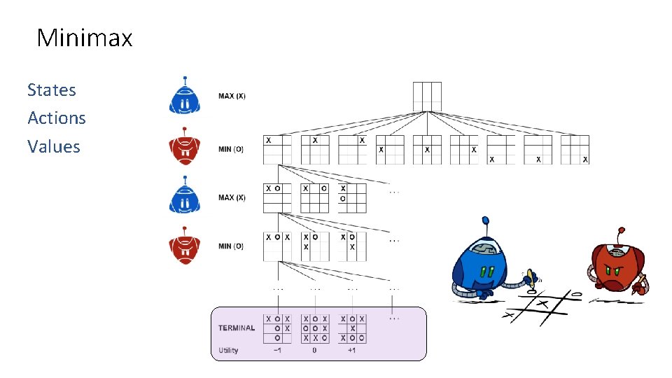
Minimax States Actions Values

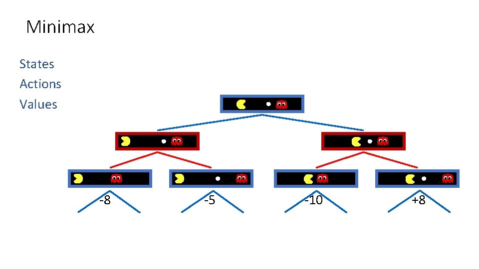
Minimax States Actions Values -8 -5 -10 +8

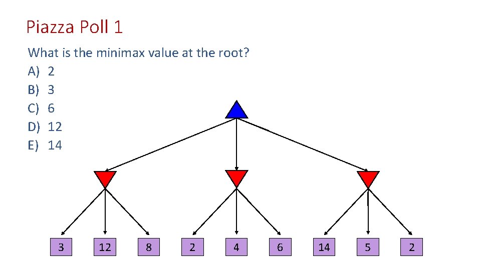
Piazza Poll 1 What is the minimax value at the root? A) 2 B) 3 C) 6 D) 12 E) 14 3 12 8 2 4 6 14 5 2

Piazza Poll 1 What is the minimax value at the root? A) 2 B) 3 C) 6 D) 12 E) 14 3 12 8 2 4 6 14 5 2

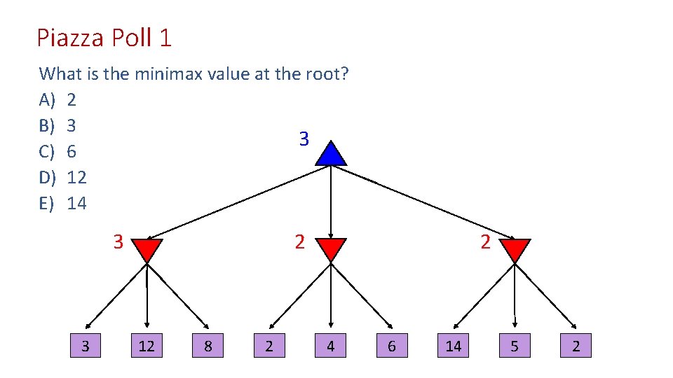
Piazza Poll 1 What is the minimax value at the root? A) 2 B) 3 3 C) 6 D) 12 E) 14 3 3 2 12 8 2 2 4 6 14 5 2

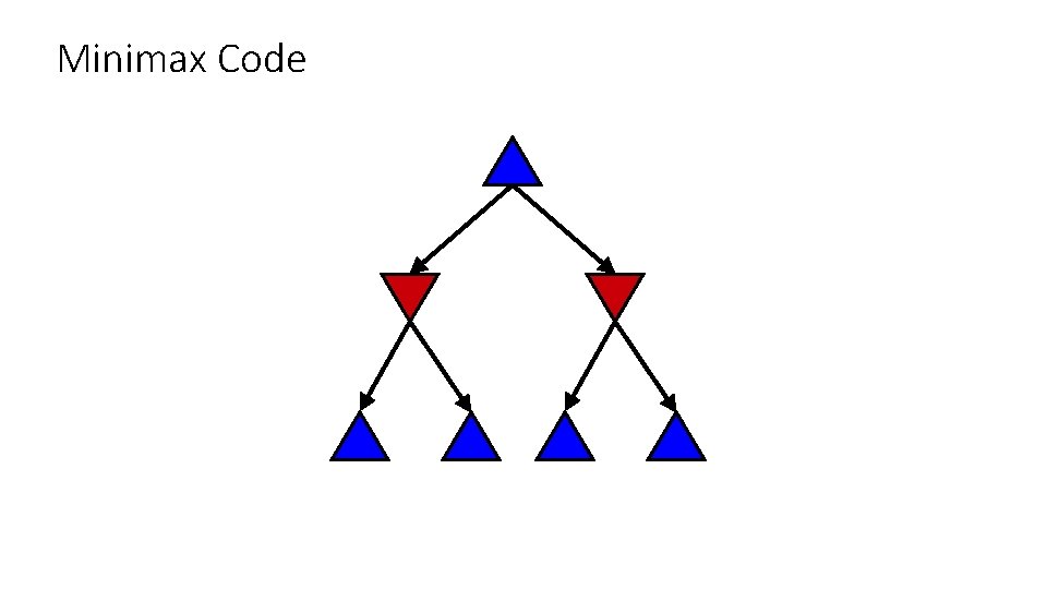
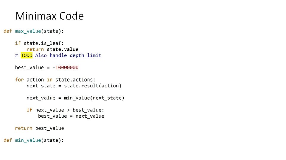
Minimax Code

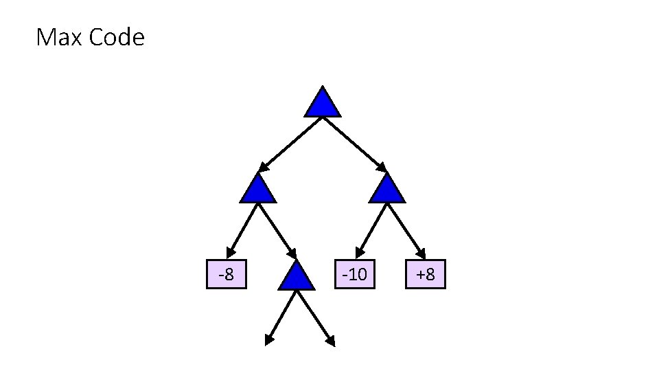
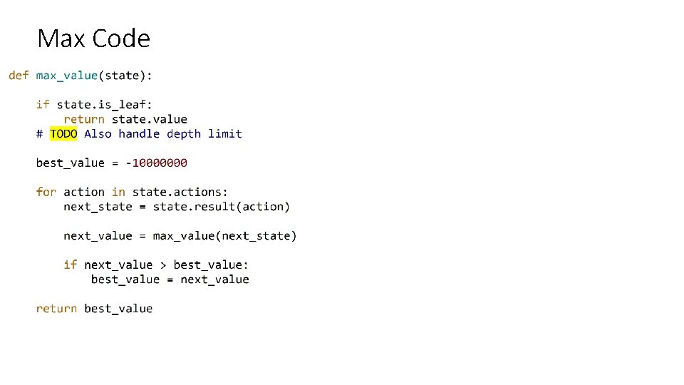
Max Code -8 -10 +8

Max Code

Minimax Code

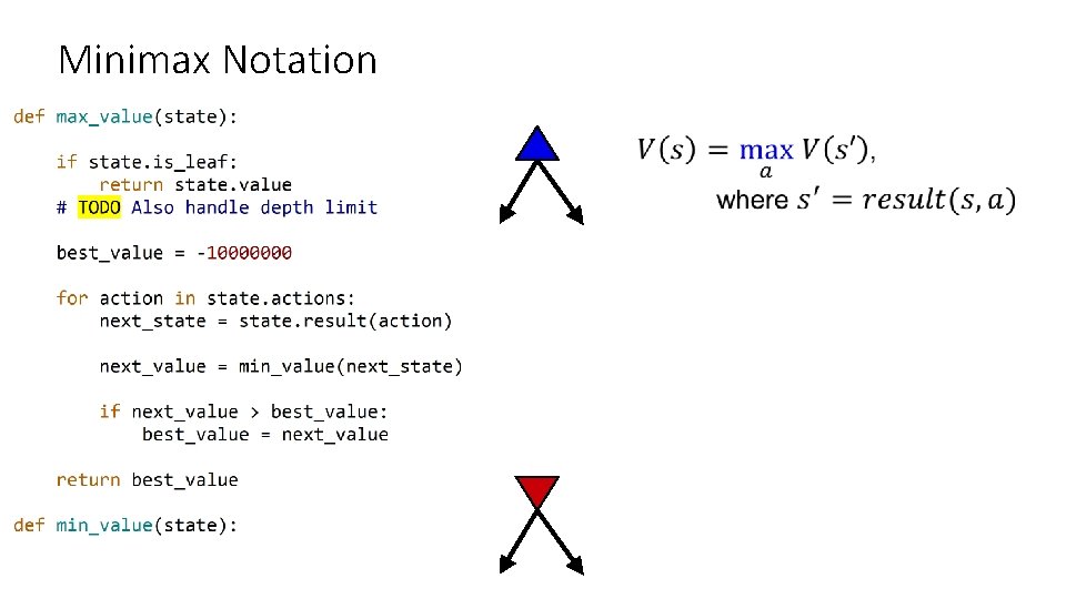
Minimax Notation

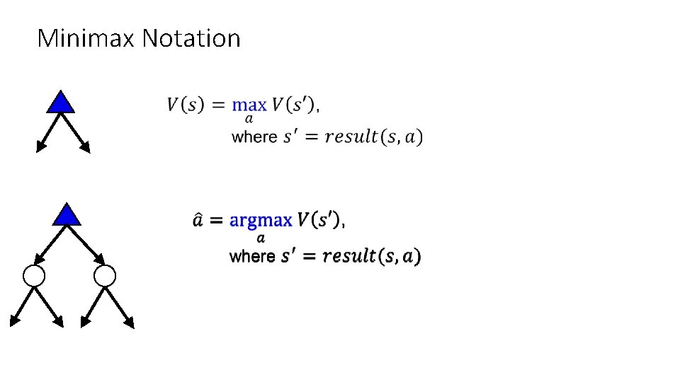
Minimax Notation

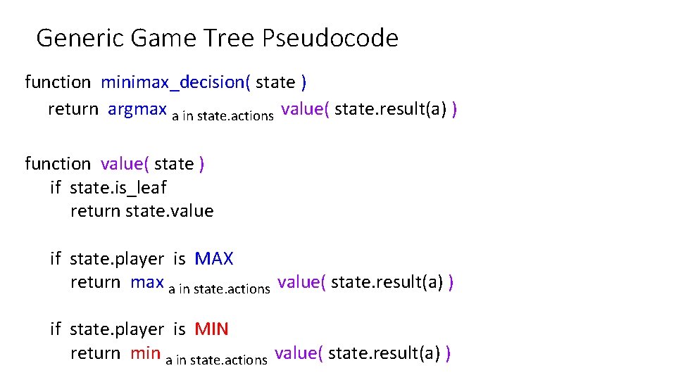
Generic Game Tree Pseudocode function minimax_decision( state ) return argmax a in state. actions value( state. result(a) ) function value( state ) if state. is_leaf return state. value if state. player is MAX return max a in state. actions value( state. result(a) ) if state. player is MIN return min a in state. actions value( state. result(a) )

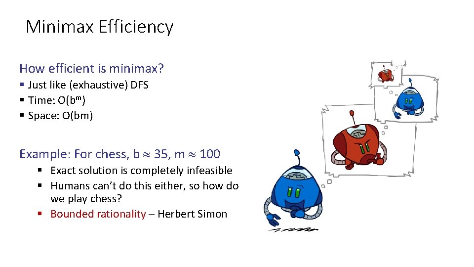
Minimax Efficiency How efficient is minimax? § Just like (exhaustive) DFS § Time: O(bm) § Space: O(bm) Example: For chess, b 35, m 100 § Exact solution is completely infeasible § Humans can’t do this either, so how do we play chess? § Bounded rationality – Herbert Simon

Resource Limits

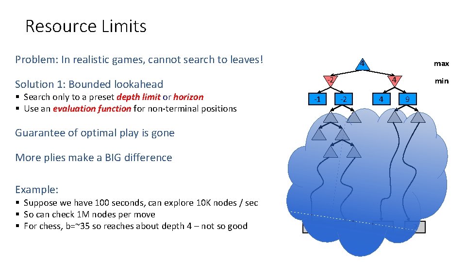
Resource Limits Problem: In realistic games, cannot search to leaves! -2 Solution 1: Bounded lookahead § Search only to a preset depth limit or horizon § Use an evaluation function for non-terminal positions max 4 -1 4 -2 4 ? ? min 9 Guarantee of optimal play is gone More plies make a BIG difference Example: § Suppose we have 100 seconds, can explore 10 K nodes / sec § So can check 1 M nodes per move § For chess, b=~35 so reaches about depth 4 – not so good ? ?

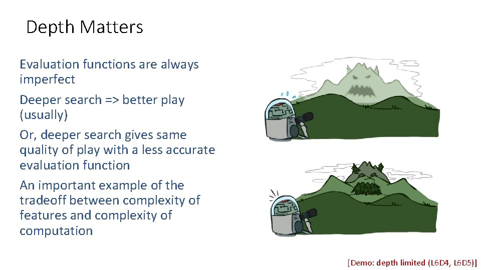
Depth Matters Evaluation functions are always imperfect Deeper search => better play (usually) Or, deeper search gives same quality of play with a less accurate evaluation function An important example of the tradeoff between complexity of features and complexity of computation [Demo: depth limited (L 6 D 4, L 6 D 5)]

Demo Limited Depth (2)

Demo Limited Depth (10)

Evaluation Functions

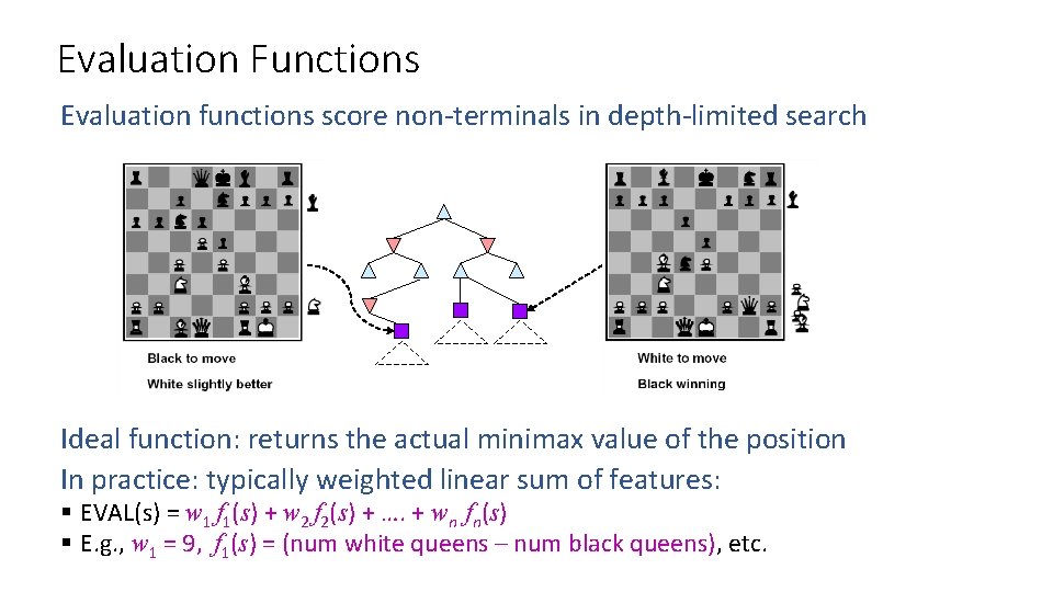
Evaluation Functions Evaluation functions score non-terminals in depth-limited search Ideal function: returns the actual minimax value of the position In practice: typically weighted linear sum of features: § EVAL(s) = w 1 f 1(s) + w 2 f 2(s) + …. + wn fn(s) § E. g. , w 1 = 9, f 1(s) = (num white queens – num black queens), etc.

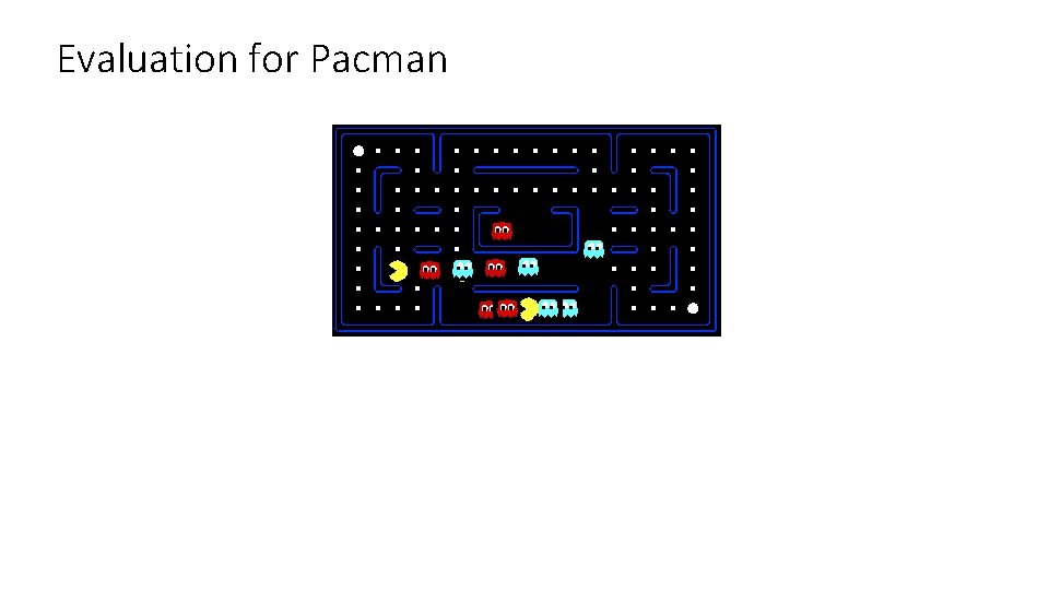
Evaluation for Pacman

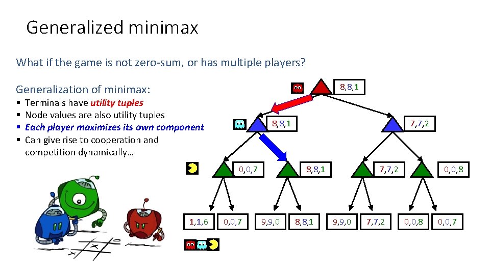
Generalized minimax What if the game is not zero-sum, or has multiple players? 8, 8, 1 Generalization of minimax: § § Terminals have utility tuples Node values are also utility tuples Each player maximizes its own component Can give rise to cooperation and competition dynamically… 8, 8, 1 0, 0, 7 1, 1, 6 0, 0, 7 7, 7, 2 8, 8, 1 9, 9, 0 8, 8, 1 7, 7, 2 9, 9, 0 7, 7, 2 0, 0, 8 0, 0, 7

Generalized minimax Three Person Chess

Game Tree Pruning

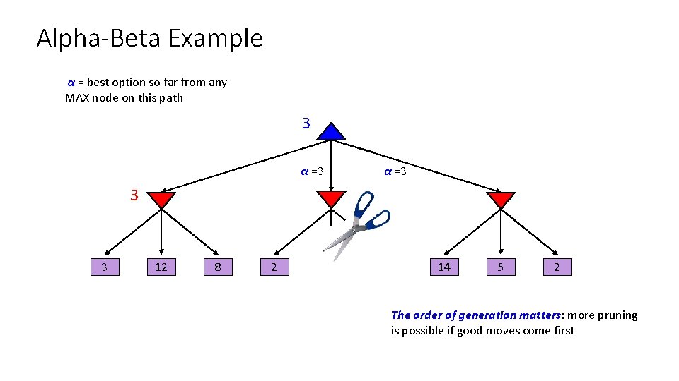
Alpha-Beta Example α = best option so far from any MAX node on this path 3 α =3 3 3 12 8 2 14 5 2 The order of generation matters: more pruning is possible if good moves come first

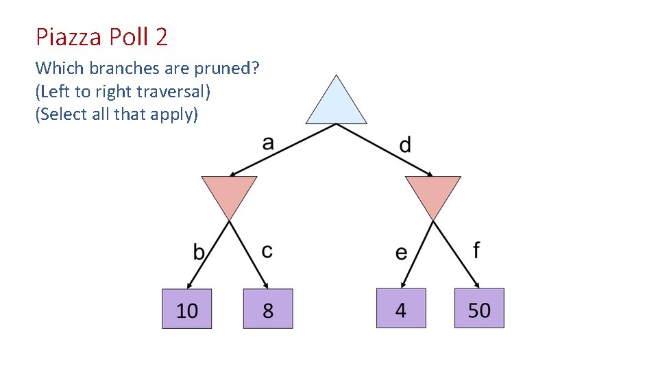
Piazza Poll 2 Which branches are pruned? (Left to right traversal) (Select all that apply)

Piazza Poll 2 Which branches are pruned? (Left to right traversal) (Select all that apply)

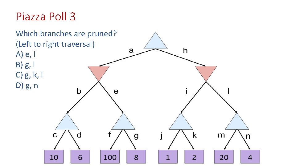
Piazza Poll 3 Which branches are pruned? (Left to right traversal) A) e, l B) g, l C) g, k, l D) g, n

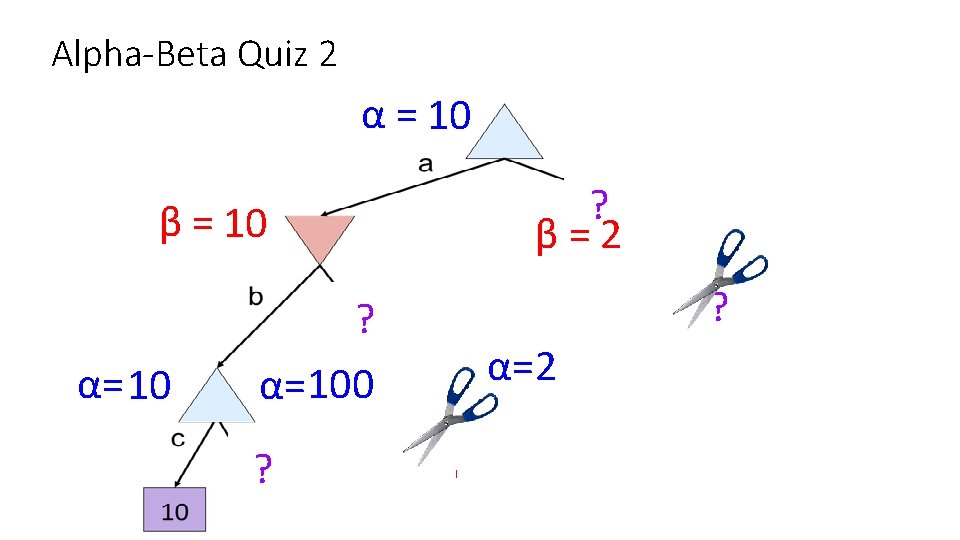
Alpha-Beta Quiz 2 α = 10 ? β=2 β = 10 α= 10 ? ? α=100 ? α=2 1 ? ?

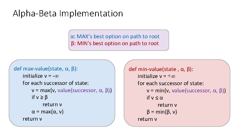
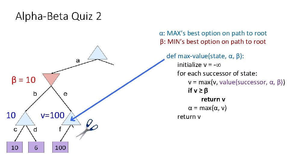
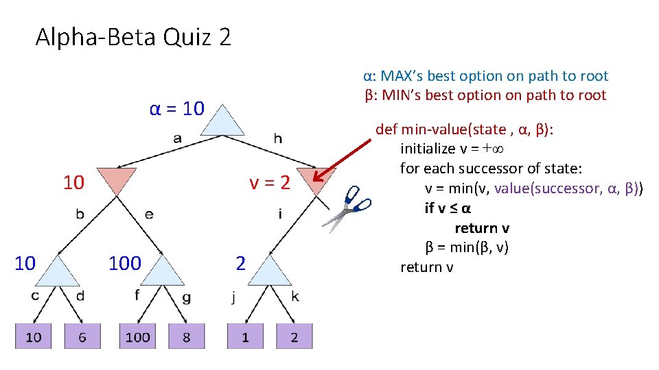
Alpha-Beta Implementation α: MAX’s best option on path to root β: MIN’s best option on path to root def max-value(state, α, β): initialize v = -∞ for each successor of state: v = max(v, value(successor, α, β)) if v ≥ β return v α = max(α, v) return v def min-value(state , α, β): initialize v = +∞ for each successor of state: v = min(v, value(successor, α, β)) if v ≤ α return v β = min(β, v) return v

Alpha-Beta Quiz 2 α: MAX’s best option on path to root β: MIN’s best option on path to root β = 10 10 v=100 def max-value(state, α, β): initialize v = -∞ for each successor of state: v = max(v, value(successor, α, β)) if v ≥ β return v α = max(α, v) return v

Alpha-Beta Quiz 2 α: MAX’s best option on path to root β: MIN’s best option on path to root α = 10 10 10 v=2 100 2 def min-value(state , α, β): initialize v = +∞ for each successor of state: v = min(v, value(successor, α, β)) if v ≤ α return v β = min(β, v) return v

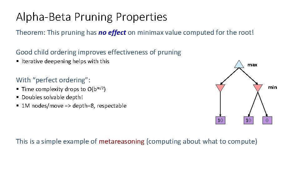
Alpha-Beta Pruning Properties Theorem: This pruning has no effect on minimax value computed for the root! Good child ordering improves effectiveness of pruning § Iterative deepening helps with this max With “perfect ordering”: min § Time complexity drops to O(bm/2) § Doubles solvable depth! § 1 M nodes/move => depth=8, respectable 10 10 This is a simple example of metareasoning (computing about what to compute) 0

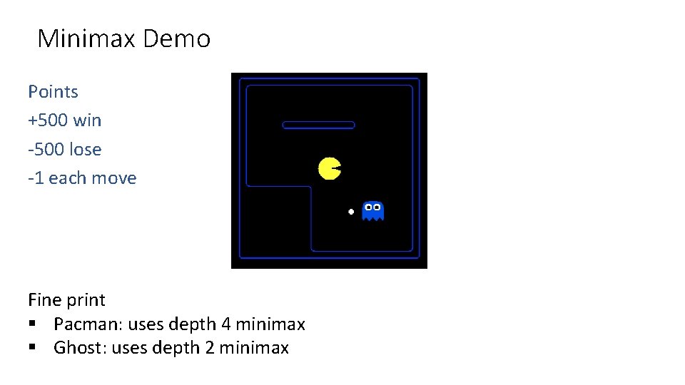
Minimax Demo Points +500 win -500 lose -1 each move Fine print § Pacman: uses depth 4 minimax § Ghost: uses depth 2 minimax

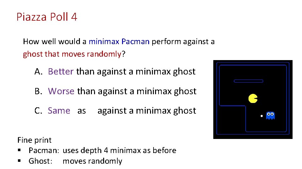
Piazza Poll 4 How well would a minimax Pacman perform against a ghost that moves randomly? A. Better than against a minimax ghost B. Worse than against a minimax ghost C. Same as against a minimax ghost Fine print § Pacman: uses depth 4 minimax as before § Ghost: moves randomly

Demo

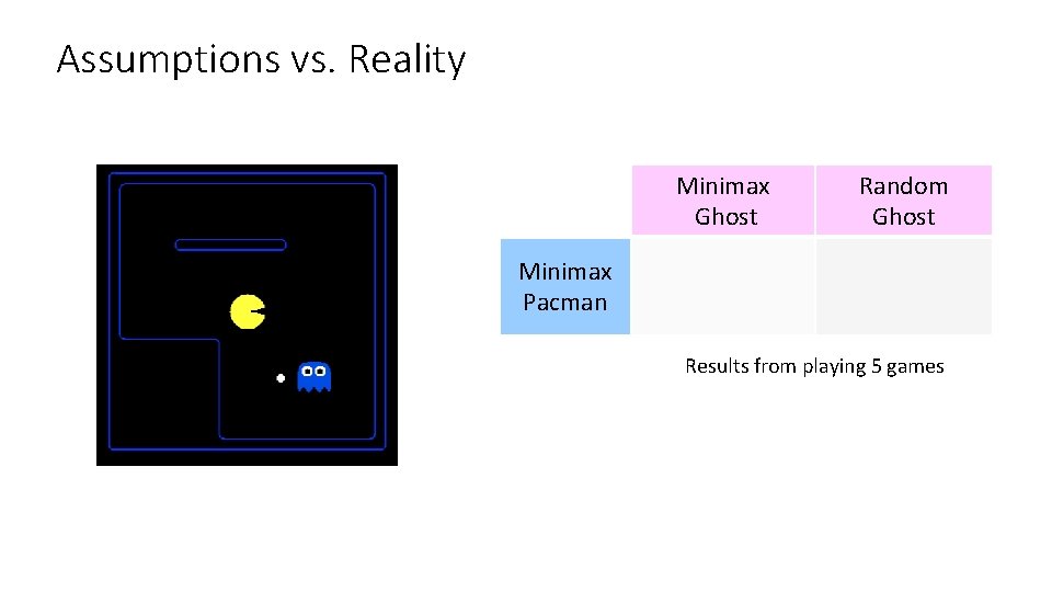
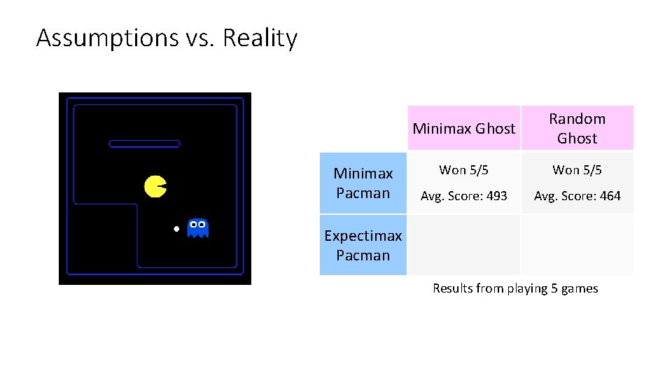
Assumptions vs. Reality Minimax Pacman Expectimax Pacman Minimax Ghost Random Ghost Won 5/5 Avg. Score: 493 Avg. Score: 464 Won 1/5 from playing Won 5/5 Results 5 games Avg. Score: -303 Avg. Score: 503

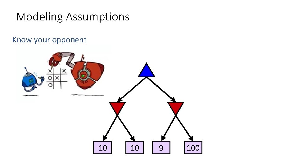
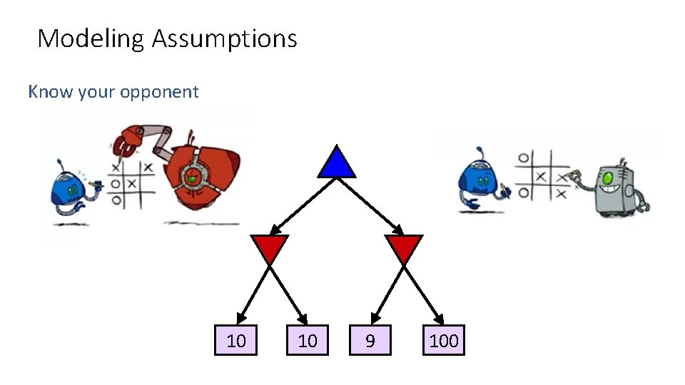
Modeling Assumptions Know your opponent 10 10 9 100

Modeling Assumptions Know your opponent 10 10 9 100

Modeling Assumptions Minimax autonomous vehicle? Image: https: //corporate. ford. com/innovation/autonomous-2021. html

Minimax Driver? Clip: How I Met Your Mother, CBS

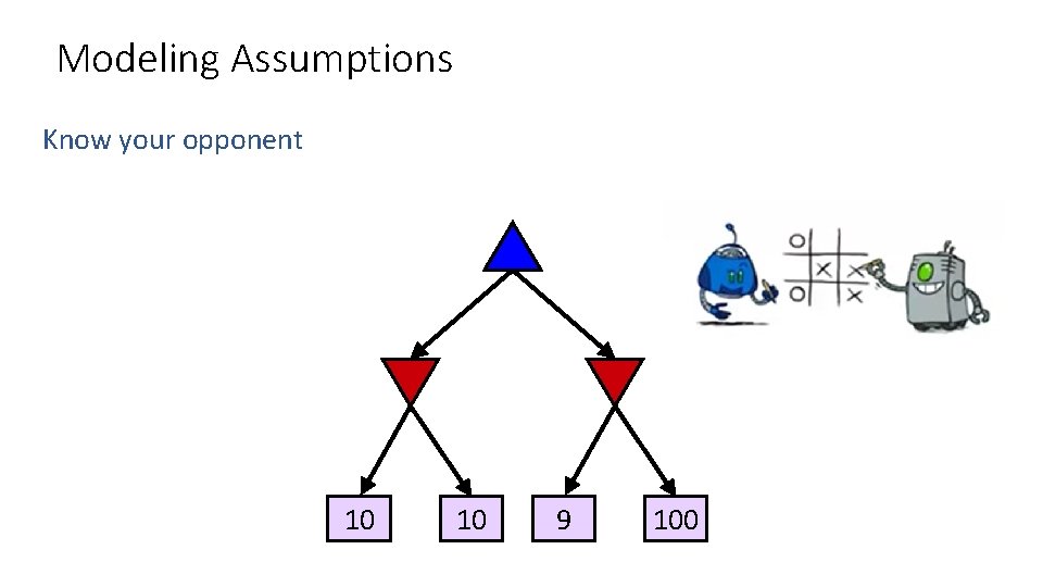
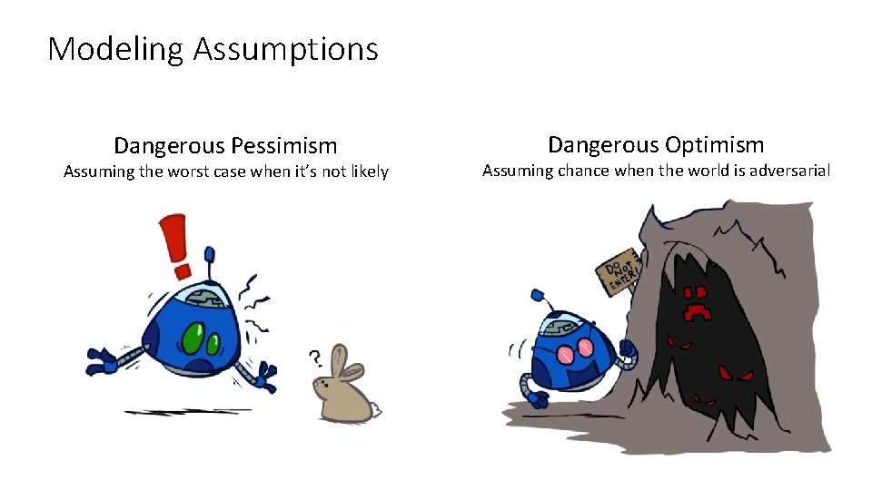
Modeling Assumptions Dangerous Pessimism Assuming the worst case when it’s not likely Dangerous Optimism Assuming chance when the world is adversarial

Modeling Assumptions Know your opponent 10 10 9 100

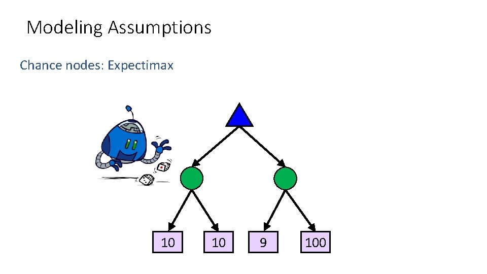
Modeling Assumptions Chance nodes: Expectimax 10 10 9 100

Assumptions vs. Reality Minimax Pacman Minimax Ghost Random Ghost Won 5/5 Avg. Score: 493 Avg. Score: 464 Won 1/5 Expectimax Pacman Avg. Score: -303 Won 5/5 Avg. Score: 503 Results from playing 5 games

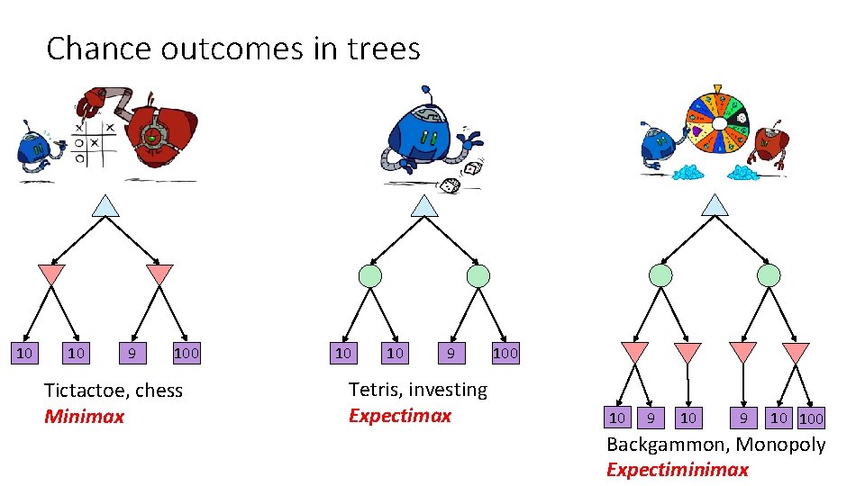
Chance outcomes in trees 10 10 9 100 Tictactoe, chess Minimax 10 10 9 Tetris, investing Expectimax 100 10 9 10 100 Backgammon, Monopoly Expectiminimax

Probabilities

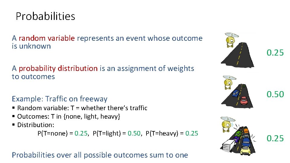
Probabilities A random variable represents an event whose outcome is unknown 0. 25 A probability distribution is an assignment of weights to outcomes Example: Traffic on freeway § Random variable: T = whethere’s traffic § Outcomes: T in {none, light, heavy} § Distribution: P(T=none) = 0. 25, P(T=light) = 0. 50, P(T=heavy) = 0. 25 Probabilities over all possible outcomes sum to one 0. 50 0. 25

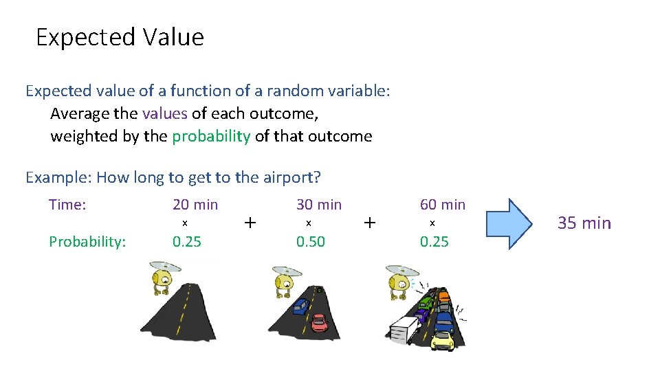
Expected Value Expected value of a function of a random variable: Average the values of each outcome, weighted by the probability of that outcome Example: How long to get to the airport? Time: 20 min x Probability: 0. 25 + 30 min x 0. 50 + 60 min x 0. 25 35 min

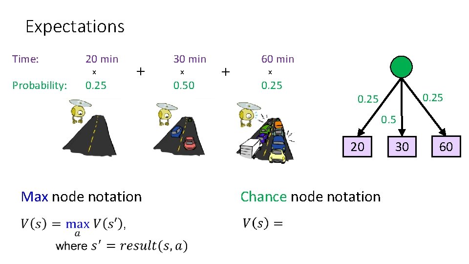
Expectations Time: 20 min x Probability: 0. 25 + 30 min x 0. 50 + 60 min x 0. 25 0. 5 20 Max node notation Chance node notation 30 60

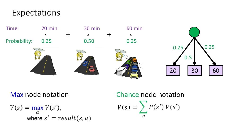
Expectations Time: 20 min x Probability: 0. 25 + 30 min x 0. 50 + 60 min x 0. 25 0. 5 20 Max node notation Chance node notation 30 60

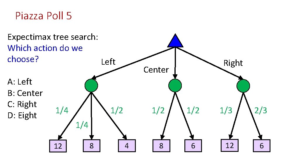
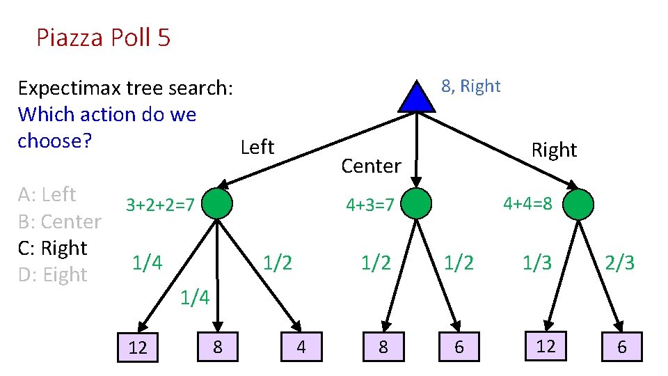
Piazza Poll 5 Expectimax tree search: Which action do we choose? Left A: Left B: Center C: Right D: Eight 1/4 Right Center 1/2 1/2 1/3 2/3 1/4 12 8 4 8 6 12 6

Piazza Poll 5 Expectimax tree search: Which action do we choose? Left A: Left B: Center C: Right D: Eight 8, Right Center 3+2+2=7 4+4=8 4+3=7 1/4 1/2 1/2 1/3 2/3 1/4 12 8 4 8 6 12 6

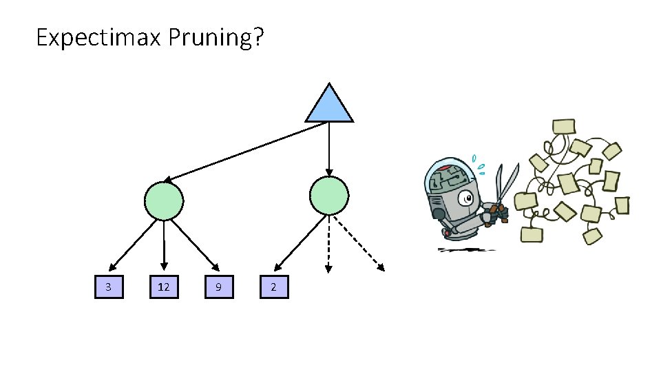
Expectimax Pruning? 3 12 9 2

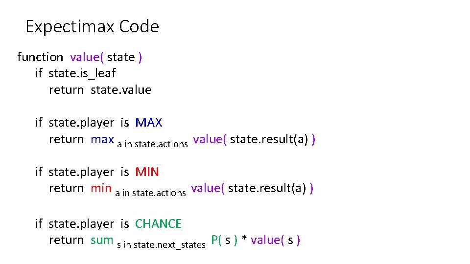
Expectimax Code function value( state ) if state. is_leaf return state. value if state. player is MAX return max a in state. actions value( state. result(a) ) if state. player is MIN return min a in state. actions value( state. result(a) ) if state. player is CHANCE return sum s in state. next_states P( s ) * value( s )

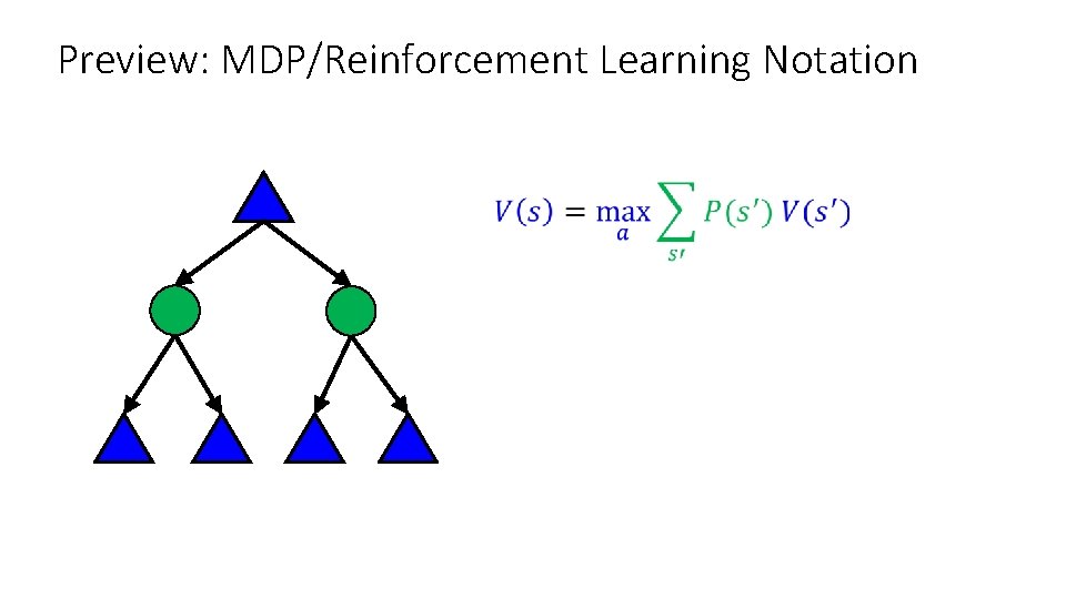
Preview: MDP/Reinforcement Learning Notation

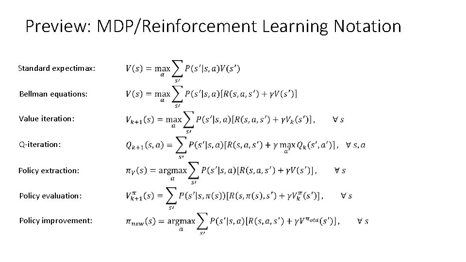
Preview: MDP/Reinforcement Learning Notation Standard expectimax: Bellman equations: Value iteration: Q-iteration: Policy extraction: Policy evaluation: Policy improvement:

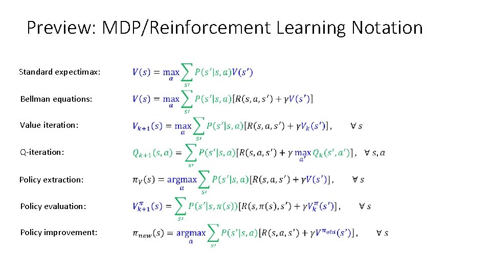
Preview: MDP/Reinforcement Learning Notation Standard expectimax: Bellman equations: Value iteration: Q-iteration: Policy extraction: Policy evaluation: Policy improvement:

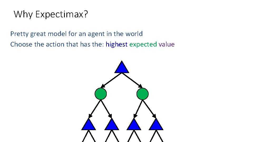
Why Expectimax? Pretty great model for an agent in the world Choose the action that has the: highest expected value

Bonus Question Let’s say you know that your opponent is actually running a depth 1 minimax, using the result 80% of the time, and moving randomly otherwise Question: What tree search should you use? A: Minimax B: Expectimax C: Something completely different

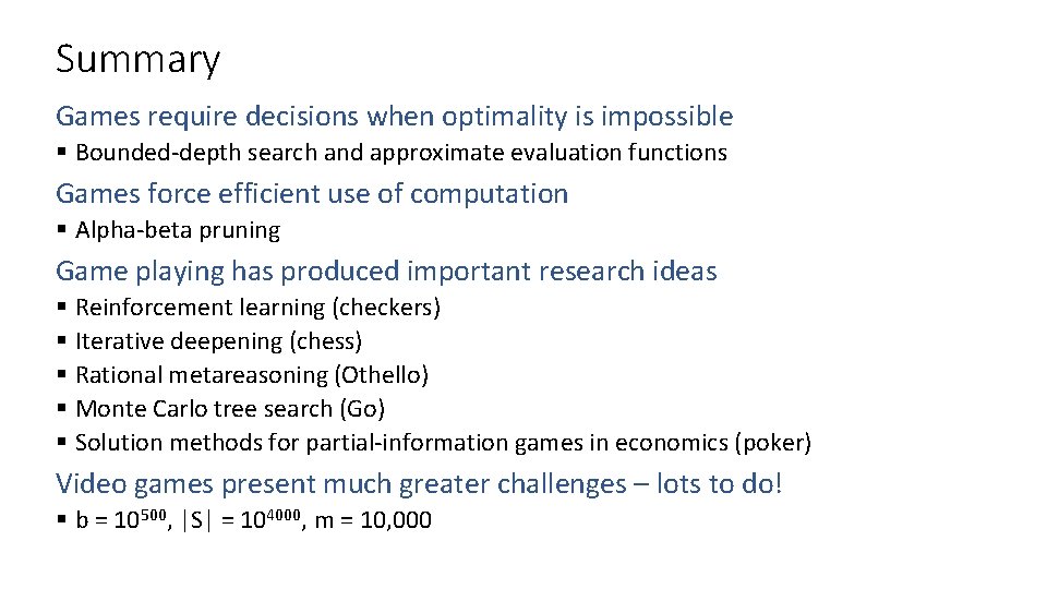
Summary Games require decisions when optimality is impossible § Bounded-depth search and approximate evaluation functions Games force efficient use of computation § Alpha-beta pruning Game playing has produced important research ideas § Reinforcement learning (checkers) § Iterative deepening (chess) § Rational metareasoning (Othello) § Monte Carlo tree search (Go) § Solution methods for partial-information games in economics (poker) Video games present much greater challenges – lots to do! § b = 10500, |S| = 104000, m = 10, 000