ANKARA UNIVERSITY DEPARTMENT OF ENERGY ENGINEERING NUMERICAL METHODS

ANKARA UNIVERSITY DEPARTMENT OF ENERGY ENGINEERING NUMERICAL METHODS INSTRUCTOR DR. ÖZGÜR SELİMOĞLU

CONTENTS Ø Numerical Integration a) Newton-Cotes Formulas b) Romberg and Gaussian Integration

Numerical Integration Numerical integration, also known as quadrature, is intrinsically a much more accurate procedure than numerical differentiation. Quadrature approximates the definite integral (1) by the sum All rules of quadrature are derived from polynomial interpolation of the integrand. Therefore, they work best if f (x) can be approximated by a polynomial. Methods of numerical integration can be divided into two groups: Newton-Cotes formulas and Gaussian quadrature. They are most useful if f (x) has already been computed at equal intervals. Because Newton-Cotes formulas are based on local interpolation, they require only a piecewise fit to a polynomial. Gaussian quadrature requires fewer evaluations of the integrand for a given level of precision, it is popular in cases where f (x) is hard to evaluate. Another advantage of Gaussian quadrature is its ability to handle integrable singularities, enabling us to evaluate expressions such as

Ø Newton-Cotes Formulas The Newton-Cotes formulas are the most common numerical integration schemes. They are based on the strategy of replacing a complicated function or tabulated data with an approximating function that is easy to integrate: (1) where fn(x) = a polynomial of the form where n is the order of the polynomial. For example, in Fig. 1. a, a first-order polynomial (a straight line) is used as an approximation. In Fig. 1. b, a parabola is employed for the same purpose. The integral can also be approximated using a series of polynomials applied piecewise to the function or data over segments of constant length. For example, in Fig. 2, three straight-line segments are used to approximate the integral. Higher-order polynomials can be utilized for the same purpose. Figure 2: The approximation of an integral by the area under three straight-line segments. Figure 1: The approximation of an integral by the area under (a) a single straight line and (b) a single parabola.

Trapezoidal Rule The trapezoidal rule is the first of the Newton-Cotes closed integration formulas. It corresponds to the case where the polynomial in Eq. (1) is first-order: From the linear interpolation formula, it is represented as the Eq. formula of a straight line; (2) The area under this straight line is an estimate of the integral of f (x) between the limits a and b: The result of the integration is; (3) which is called the trapezoidal rule.

Geometrically, the trapezoidal rule is equivalent to approximating the area of the trapezoid under the straight line connecting f (a) and f (b) in Fig. 3. Recall from geometry that the formula for computing the area of a trapezoid is the height times the average of the bases (Fig. 4. a). In our case, the concept is the same but the trapezoid is on its side (Fig. 4. b). Therefore, the integral estimate can be represented as (4) Figure 3: Graphical depiction of the trapezoidal rule. or (5) where, for the trapezoidal rule, the average height is the average of the function values at the end points, or [ f (a) + f (b)]/2. All the Newton-Cotes closed formulas can be expressed in the general format of Eq. (4). Figure 4: (a) The formula for computing the area of a trapezoid: height times the average of the bases. (b) For the trapezoidal rule, the concept is the same but the trapezoid is on its side.

Error of the Trapezoidal Rule When we employ the integral under a straight-line segment to approximate the integral under a curve, we obviously can experience an error that may be substantial (Fig. 5). An estimate for the local truncation error of a single application of the trapezoidal rule is (Box. 1) (6) where ξ lies somewhere in the interval from a to b. Equation (6) indicates that if the function being integrated is linear, the trapezoidal rule will be exact. Otherwise, for functions with second- and higher-order derivatives (that is, with curvature), some error can occur. Figure 5: Graphical depiction of the use of a single application of the trapezoidal rule to approximate the integral of, f(x) = 0. 2 + 25 x − 200 x 2 + 675 x 3 − 900 x 4 + 400 x 5 from x = 0 to 0. 8. Box 1: Derivation and Error Estimate of the Trapezoidal Rule

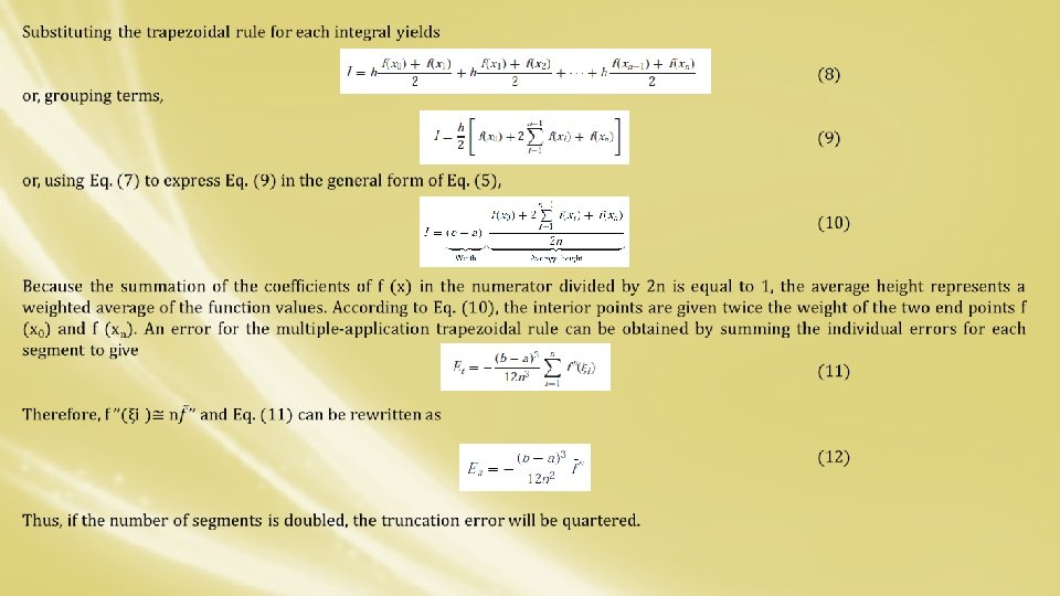
The Multiple-Application Trapezoidal Rule One way to improve the accuracy of the trapezoidal rule is to divide the integration interval from a to b into a number of segments and apply the method to each segment (Fig. 6). The areas of individual segments can then be added to yield the integral for the entire interval. The resulting equations are called multiple-application, or composite, integration formulas. Figure 7 shows the general format and nomenclature we will use to characterize multiple-application integrals. There are n + 1 equally spaced base points (x 0, x 1, x 2, . . . , xn). Consequently, there are n segments of equal width: (7) Figure 6: Illustration of the multipleapplication trapezoidal rule. (a) Two segments, (b) three segments, (c) four segments, and (d) five segments. If a and b are designated as x 0 and xn, respectively, the total integral can be represented as Figure 7: The general format and nomenclature for multipleapplication integrals.

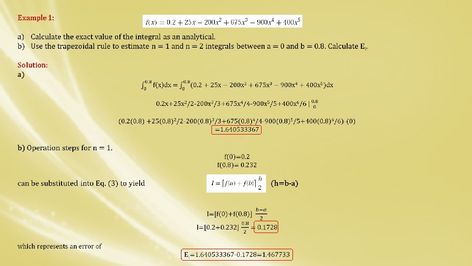
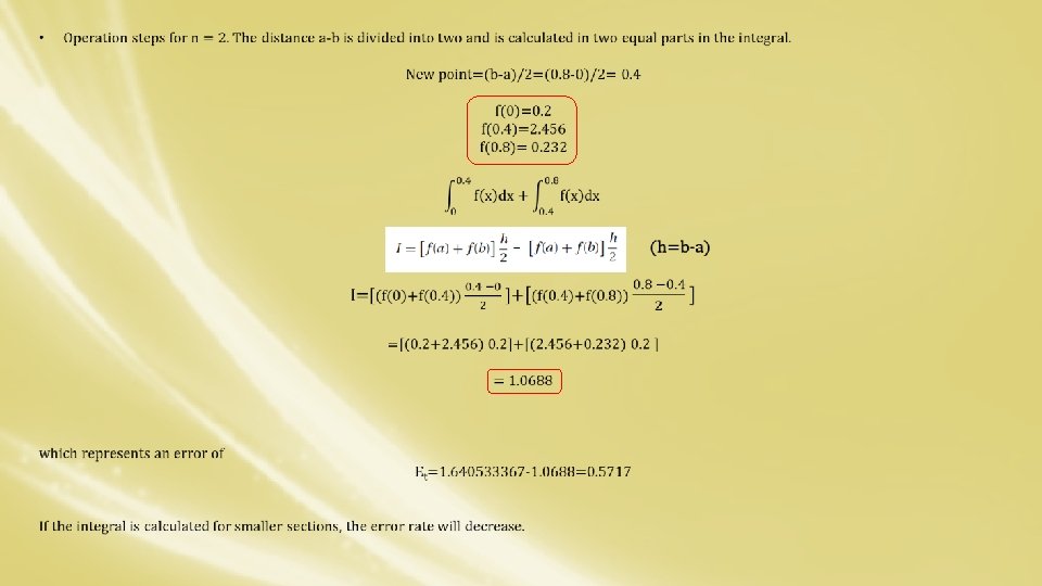
For n=1 to a percent relative error is ε t = 89. 5%. The reason for this large error is evident from the graphical depiction in Fig. (5). Notice that the area under the straight line neglects a significant portion of the integral lying above the line. In actual situations, we would have no foreknowledge of the true value. Therefore, an approximate error estimate is required. To obtain this estimate, the function’s second derivative over the interval can be computed by differentiating the original function twice to give The average value of the second derivative can be computed using Eq. : which can be substituted into Eq. (5) to yield which is of the same order of magnitude and sign as the true error. A discrepancy does exist, however, because of the fact that for an interval of this size, the average second derivative is not necessarily an accurate approximation of f (ξ). Thus, we denote that the error is approximate by using the notation E a, rather than exact by using Et.

Ø Simpson’s Rules Aside from applying the trapezoidal rule with finer segmentation, another way to obtain a more accurate estimate of an integral is to use higher-order polynomials to connect the points. For example, if there is an extra point midway between f (a) and f (b), the three points can be connected with a parabola (Fig. 6. a). If there are two points equally spaced between f (a) and f (b), the four points can be connected with a third-order polynomial (Fig. 6. b). The formulas that result from taking the integrals under these polynomials are called Simpson’s rules. Simpson’s 1/3 Rule Simpson’s 1/3 rule results when a second-order interpolating polynomial is substituted into Eq. (1): (13) If a and b are designated as x 0 and x 2 and f 2(x) is represented by a second-order Lagrange polynomial [Eq. ]the integral becomes Figure 6: (a) Graphical depiction of Simpson’s 1/3 rule: It consists of taking the area under a parabola connecting three points. (b) Graphical depiction of Simpson’s 3/8 rule: It consists of taking the area under a cubic equation connecting four points.

After integration and algebraic manipulation, the following formula results: (14) where, for this case, h = (b − a)/2. This equation is known as Simpson’s 1/3 rule. It is the second Newton-Cotes closed integration formula. The label “ 1/3” stems from the fact that h is divided by 3 in Eq. (14). An alternative derivation is shown in Box 2 where the Newton-Gregory polynomial is integrated to obtain the same formula. Simpson’s 1/3 rule can also be expressed using the format of Eq. (5): (15) Box 2 : Derivation and Error Estimate of Simpson’s 1/3 Rule

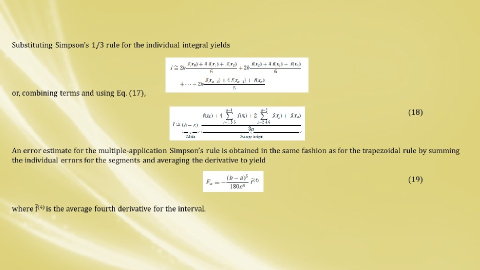
where a = x 0, b = x 2, and x 1 = the point midway between a and b, which is given by (b + a)/2. Notice that, according to Eq. (15), the middle point is weighted by two-thirds and the two end points by one-sixth. It can be shown that a single-segment application of Simpson’s 1/3 rule has a truncation error of (Box 2) or, because h = (b − a)/2, (16) where ξ lies somewhere in the interval from a to b. Thus, Simpson’s 1/3 rule is more accurate than the trapezoidal rule. However, comparison with Eq. (6) indicates that it is more accurate than expected. Rather than being proportional to the third derivative, the error is proportional to the fourth derivative. The Multiple-Application Simpson’s 1/3 Rule Just as with the trapezoidal rule, Simpson’s rule can be improved by dividing the integration interval into a number of segments of equal width (Fig. 7): (17) The total integral can be represented as Figure 7 : Graphical representation of the multiple application of Simpson’s 1/3 rule.

Simpson’s 3/8 Rule In a similar manner to the derivation of the trapezoidal and Simpson’s 1/3 rule, a third order Lagrange polynomial can be fit to four points and integrated: where h = (b − a)/3. This equation is called Simpson’s 3/8 rule because h is multiplied by 3/8. It is the third Newton-Cotes closed integration formula. The 3/8 rule can also be expressed in the form of Eq. (5): (20) Thus, the two interior points are given weights of three-eighths, whereas the end points are weighted with one-eighth. Simpson’s 3/8 rule has an error of Figure 8 : Illustration of how Simpson’s 1/3 and 3/8 rules can be applied in tandem to handle multiple applications with odd numbers of intervals. (21) Simpson’s 1/3 rule is usually the method of preference because it attains third-order accuracy with three points rather than the four points required for the 3/8 version. However, the 3/8 rule has utility when the number of segments is odd.

Example 2 : Use Eq. (E. 2) with n = 4 to estimate the integral of. from a = 0 to b = 0. 8. Recall that the exact integral is 1. 640533. Solution: • n = 4 (h = 0. 2): From Eq. (E. 2) , (E. 2) The estimated error [Eq. (E. 2. a)] is (E. 2. a)

REFERENCES • Jaan Kiusalaas, “Numerical Methods in Engineering with Python 3”, 3 rd Edition, Cambridge, NY, 2013 • S. C. Chapra and R. P. Canale, “Numerical Methods for Engineers”, 6 th ed. , Mc. Graw-Hill, , NY, 2010