Animation Lecture 13 Slide 1 1 Computer Animation

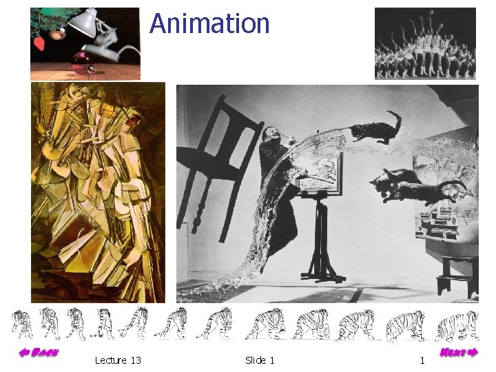
Animation Lecture 13 Slide 1 1

Computer Animation Methods Keyframing Interpolation Kinematics Inverse Kinematics Slides courtesy of Leonard Mc. Millan and Jovan Popovic Lecture 13 6. 837 Fall 2002

Administrative Assignment 6 is due Monday 28 at 5 pm n n Ray tracing Shadow, reflection, refraction Supersampling Office hours n n n Durand Thursday 4 -6 pm in 4 -035 Ngan Thursday 4 -7 in W 20 -575 Teller Friday 3 -5 in W 20 -575 Ngan Monday 10 -12 NE 43 -256 Durand Monday 2 -4 pm in NE 43 -254 Final project n n Deadline for team building: Friday Nov 1 Brainstorming session on Thursday Lecture 13 Slide 3 3

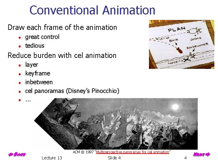
Conventional Animation Draw each frame of the animation n n great control tedious Reduce burden with cel animation n n layer keyframe inbetween cel panoramas (Disney’s Pinocchio). . . ACM © 1997 “Multiperspective panoramas for cel animation” Lecture 13 Slide 4 4

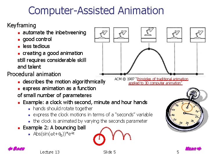
Computer-Assisted Animation Keyframing automate the inbetweening n good control n less tedious n creating a good animation still requires considerable skill and talent n Procedural animation ACM © 1987 “Principles of traditional animation describes the motion algorithmically applied to 3 D computer animation” n express animation as a function of small number of parameteres n Example: a clock with second, minute and hour hands n n n hands should rotate together express the clock motions in terms of a “seconds” variable the clock is animated by varying the seconds parameter Example 2: A bouncing ball n Abs(sin(wt+q 0))*e-kt Lecture 13 Slide 5 5

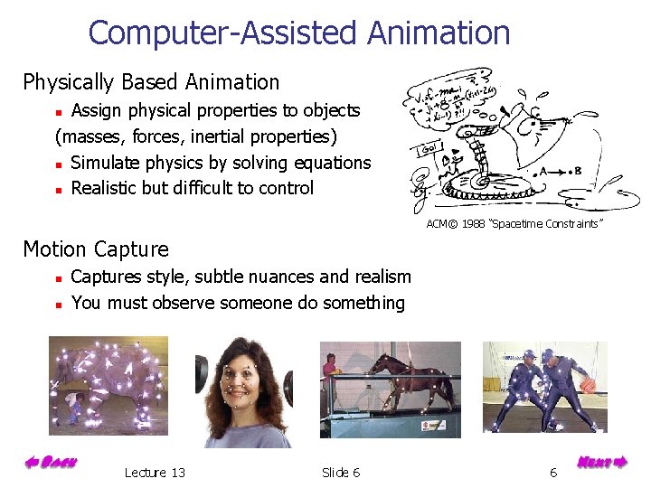
Computer-Assisted Animation Physically Based Animation Assign physical properties to objects (masses, forces, inertial properties) n Simulate physics by solving equations n Realistic but difficult to control n ACM© 1988 “Spacetime Constraints” Motion Capture n n Captures style, subtle nuances and realism You must observe someone do something Lecture 13 Slide 6 6

Overview Keyframing and interpolation Interpolation of rotations, quaternions Kimematrics, articulation Physisally-based simulation & particles Lecture 13 Slide 7 7

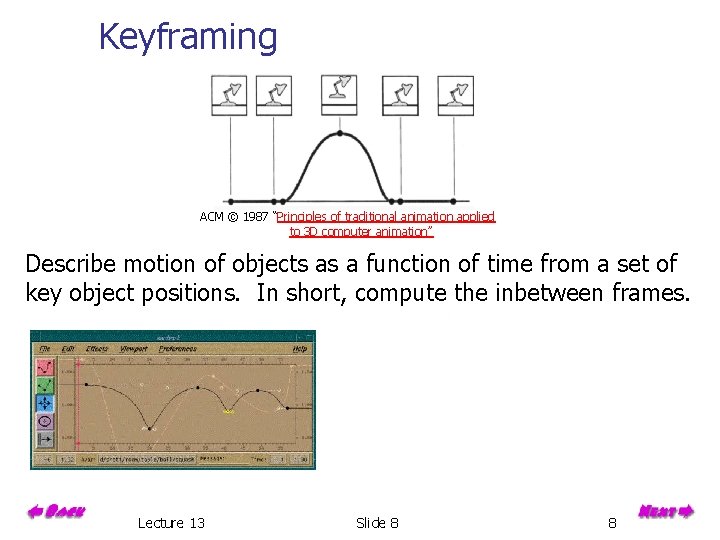
Keyframing ACM © 1987 “Principles of traditional animation applied to 3 D computer animation” Describe motion of objects as a function of time from a set of key object positions. In short, compute the inbetween frames. Lecture 13 Slide 8 8

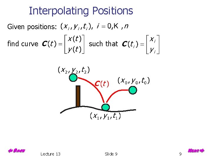
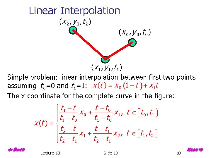
Interpolating Positions Given positions: find curve such that Lecture 13 Slide 9 9

Linear Interpolation Simple problem: linear interpolation between first two points assuming : The x-coordinate for the complete curve in the figure: Lecture 13 Slide 10 10

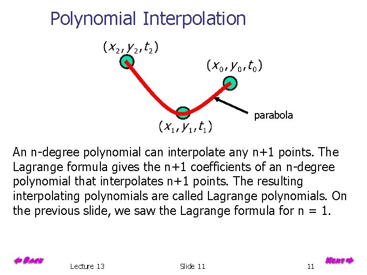
Polynomial Interpolation parabola An n-degree polynomial can interpolate any n+1 points. The Lagrange formula gives the n+1 coefficients of an n-degree polynomial that interpolates n+1 points. The resulting interpolating polynomials are called Lagrange polynomials. On the previous slide, we saw the Lagrange formula for n = 1. Lecture 13 Slide 11 11

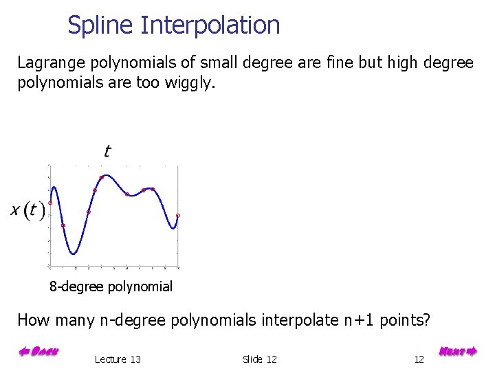
Spline Interpolation Lagrange polynomials of small degree are fine but high degree polynomials are too wiggly. 8 -degree polynomial spline vs. polynomial How many n-degree polynomials interpolate n+1 points? Lecture 13 Slide 12 12

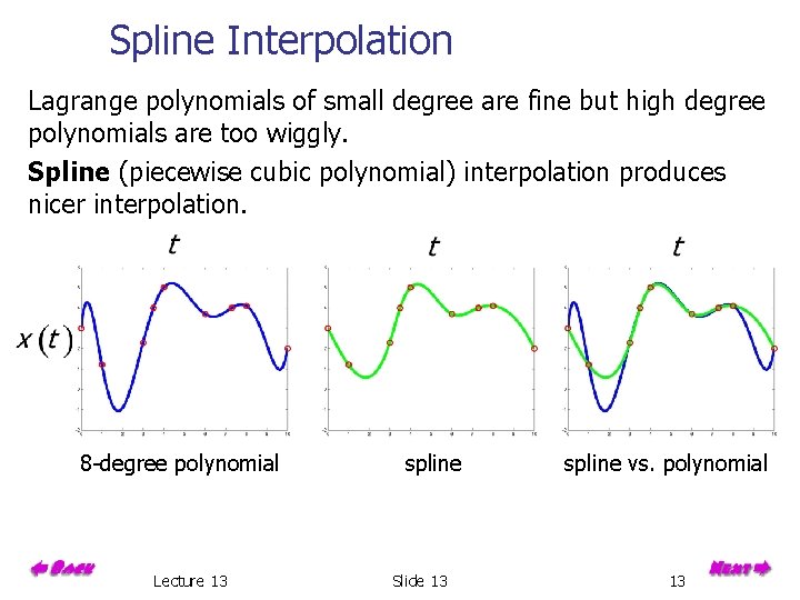
Spline Interpolation Lagrange polynomials of small degree are fine but high degree polynomials are too wiggly. Spline (piecewise cubic polynomial) interpolation produces nicer interpolation. 8 -degree polynomial Lecture 13 spline Slide 13 spline vs. polynomial 13

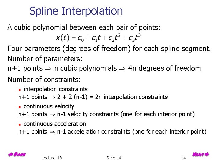
Spline Interpolation A cubic polynomial between each pair of points: Four parameters (degrees of freedom) for each spline segment. Number of parameters: n+1 points n cubic polynomials 4 n degrees of freedom Number of constraints: interpolation constraints n+1 points 2 + 2 (n-1) = 2 n interpolation constraints n continuous velocity n+1 points n-1 velocity constraints (one for each interior point) n continuous acceleration n+1 points n-1 acceleration constraints (one for each interior point) n Lecture 13 Slide 14 14

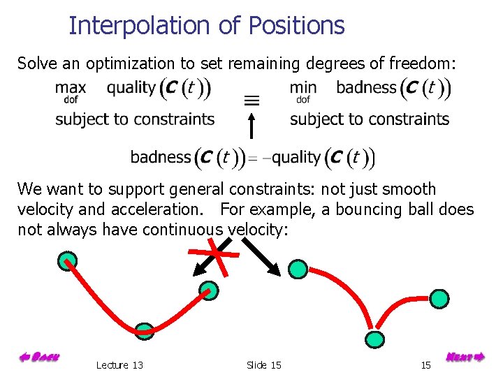
Interpolation of Positions Solve an optimization to set remaining degrees of freedom: We want to support general constraints: not just smooth velocity and acceleration. For example, a bouncing ball does not always have continuous velocity: Lecture 13 Slide 15 15

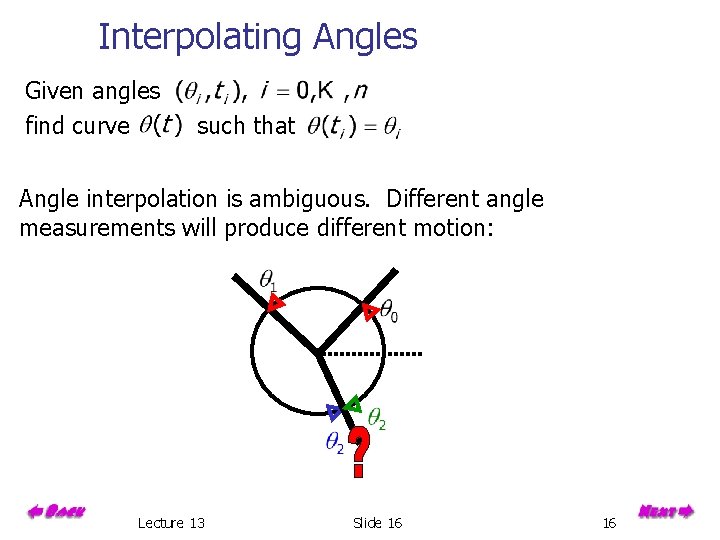
Interpolating Angles Given angles find curve such that Angle interpolation is ambiguous. Different angle measurements will produce different motion: Lecture 13 Slide 16 16

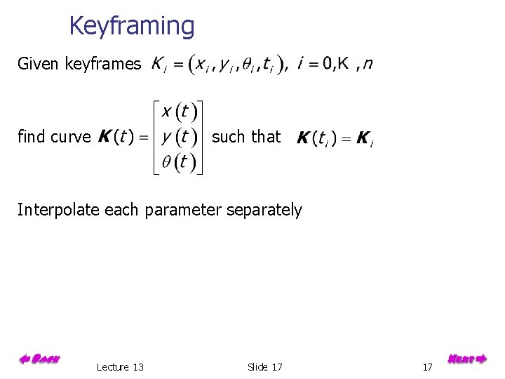
Keyframing Given keyframes find curve such that Interpolate each parameter separately Lecture 13 Slide 17 17

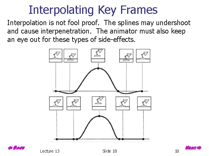
Interpolating Key Frames Interpolation is not fool proof. The splines may undershoot and cause interpenetration. The animator must also keep an eye out for these types of side-effects. Lecture 13 Slide 18 18

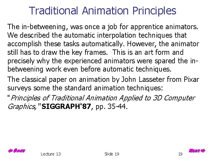
Traditional Animation Principles The in-betweening, was once a job for apprentice animators. We described the automatic interpolation techniques that accomplish these tasks automatically. However, the animator still has to draw the key frames. This is an art form and precisely why the experienced animators were spared the inbetweening work even before automatic techniques. The classical paper on animation by John Lasseter from Pixar surveys some the standard animation techniques: "Principles of Traditional Animation Applied to 3 D Computer Graphics, “ SIGGRAPH'87, pp. 35 -44. Lecture 13 Slide 19 19

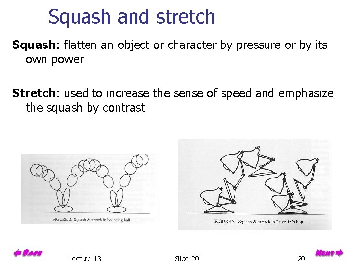
Squash and stretch Squash: flatten an object or character by pressure or by its own power Stretch: used to increase the sense of speed and emphasize the squash by contrast Lecture 13 Slide 20 20

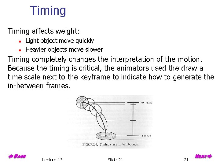
Timing affects weight: n n Light object move quickly Heavier objects move slower Timing completely changes the interpretation of the motion. Because the timing is critical, the animators used the draw a time scale next to the keyframe to indicate how to generate the in-between frames. Lecture 13 Slide 21 21

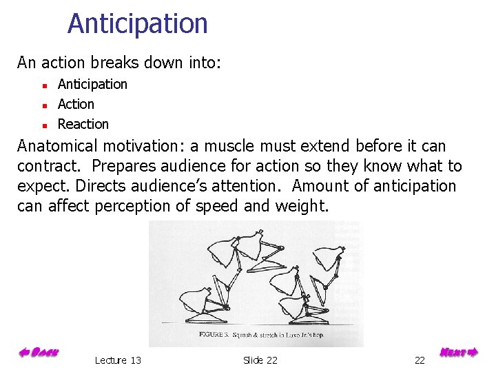
Anticipation An action breaks down into: n n n Anticipation Action Reaction Anatomical motivation: a muscle must extend before it can contract. Prepares audience for action so they know what to expect. Directs audience’s attention. Amount of anticipation can affect perception of speed and weight. Lecture 13 Slide 22 22

Overview Keyframing and interpolation Interpolation of rotations, quaternions Kimematrics, articulation Physisally-based simulation & particles Lecture 13 Slide 23 23

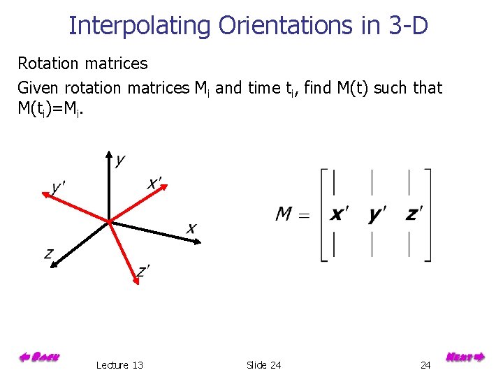
Interpolating Orientations in 3 -D Rotation matrices Given rotation matrices Mi and time ti, find M(t) such that M(ti)=Mi. Lecture 13 Slide 24 24

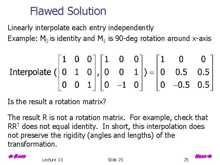
Flawed Solution Linearly interpolate each entry independently Example: M 0 is identity and M 1 is 90 -deg rotation around x-axis Is the result a rotation matrix? The result R is not a rotation matrix. For example, check that RRT does not equal identity. In short, this interpolation does not preserve the rigidity (angles and lengths) of the transformation. Lecture 13 Slide 25 25

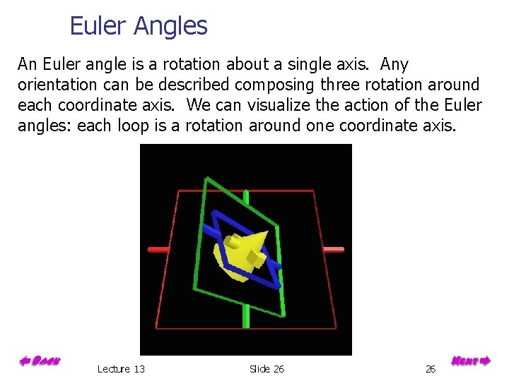
Euler Angles An Euler angle is a rotation about a single axis. Any orientation can be described composing three rotation around each coordinate axis. We can visualize the action of the Euler angles: each loop is a rotation around one coordinate axis. Lecture 13 Slide 26 26

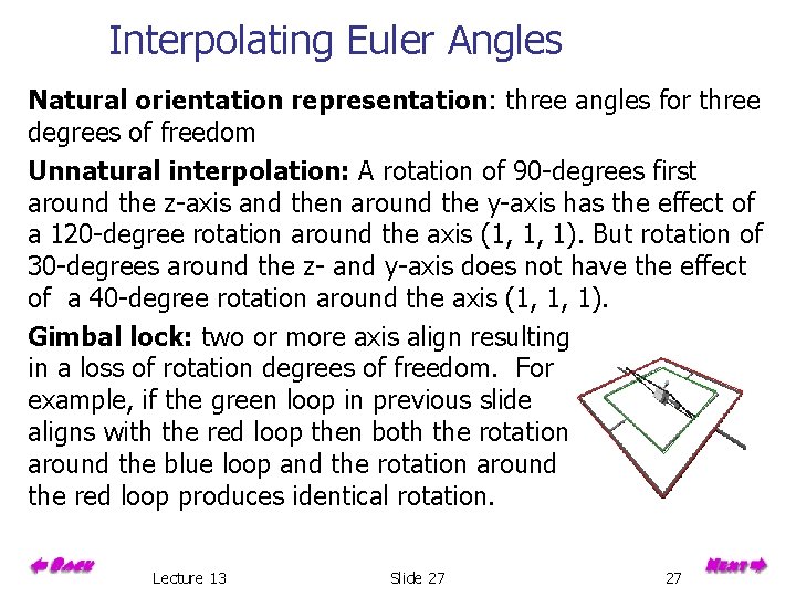
Interpolating Euler Angles Natural orientation representation: three angles for three degrees of freedom Unnatural interpolation: A rotation of 90 -degrees first around the z-axis and then around the y-axis has the effect of a 120 -degree rotation around the axis (1, 1, 1). But rotation of 30 -degrees around the z- and y-axis does not have the effect of a 40 -degree rotation around the axis (1, 1, 1). Gimbal lock: two or more axis align resulting in a loss of rotation degrees of freedom. For example, if the green loop in previous slide aligns with the red loop then both the rotation around the blue loop and the rotation around the red loop produces identical rotation. Lecture 13 Slide 27 27

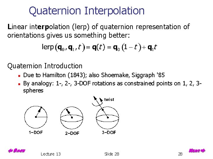
Quaternion Interpolation Linear interpolation (lerp) of quaternion representation of orientations gives us something better: Quaternion Introduction n n Due to Hamilton (1843); also Shoemake, Siggraph '85 By analogy: 1 -, 2 -, 3 -DOF rotations as constrained points on 1, 2, 3 spheres Lecture 13 Slide 28 28

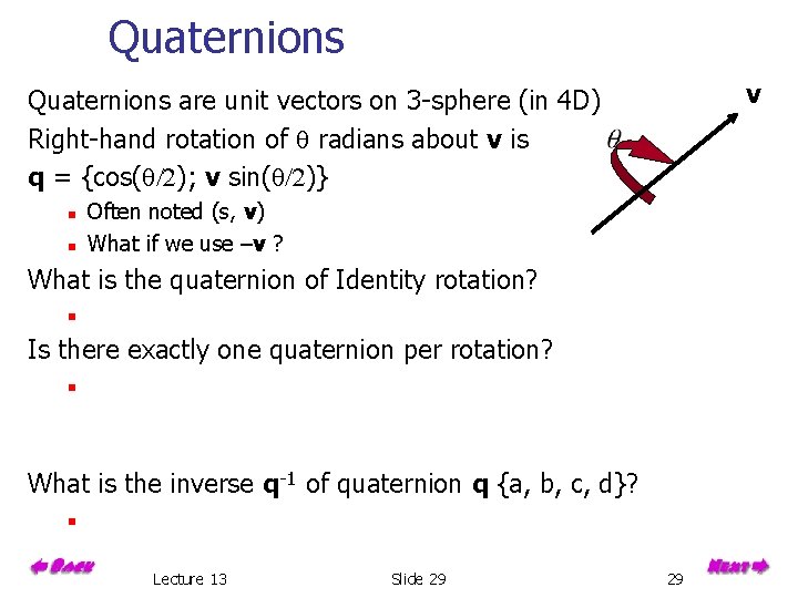
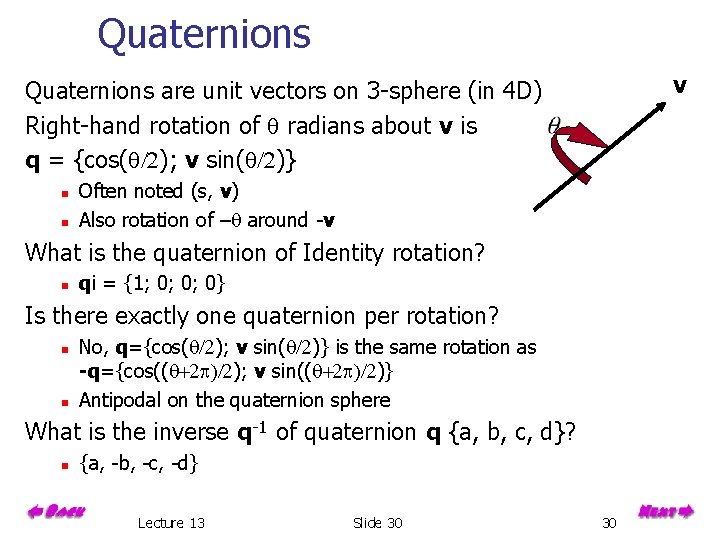
Quaternions v Quaternions are unit vectors on 3 -sphere (in 4 D) Right-hand rotation of q radians about v is q = {cos(q/2); v sin(q/2)} n n Often noted (s, v) What if we use –v ? What is the quaternion of Identity rotation? n Is there exactly one quaternion per rotation? n What is the inverse q-1 of quaternion q {a, b, c, d}? n Lecture 13 Slide 29 29

Quaternions v Quaternions are unit vectors on 3 -sphere (in 4 D) Right-hand rotation of q radians about v is q = {cos(q/2); v sin(q/2)} n n Often noted (s, v) Also rotation of –q around -v What is the quaternion of Identity rotation? n qi = {1; 0; 0; 0} Is there exactly one quaternion per rotation? n n No, q={cos(q/2); v sin(q/2)} is the same rotation as -q={cos((q+2 p)/2); v sin((q+2 p)/2)} Antipodal on the quaternion sphere What is the inverse q-1 of quaternion q {a, b, c, d}? n {a, -b, -c, -d} Lecture 13 Slide 30 30

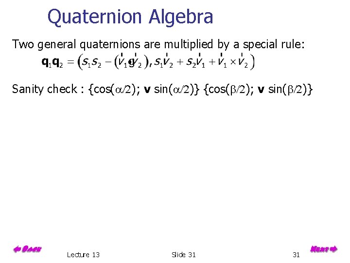
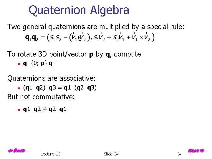
Quaternion Algebra Two general quaternions are multiplied by a special rule: Sanity check : {cos(a/2); v sin(a/2)} {cos(b/2); v sin(b/2)} Lecture 13 Slide 31 31

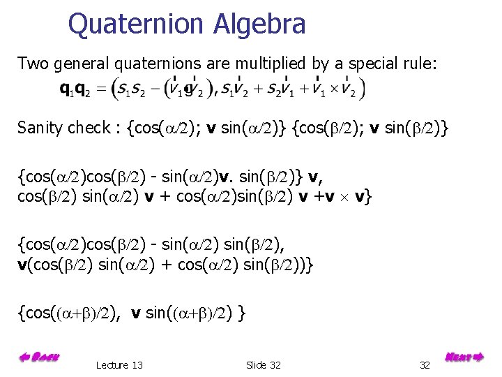
Quaternion Algebra Two general quaternions are multiplied by a special rule: Sanity check : {cos(a/2); v sin(a/2)} {cos(b/2); v sin(b/2)} {cos(a/2)cos(b/2) - sin(a/2)v. sin(b/2)} v, cos(b/2) sin(a/2) v + cos(a/2)sin(b/2) v +v v} {cos(a/2)cos(b/2) - sin(a/2) sin(b/2), v(cos(b/2) sin(a/2) + cos(a/2) sin(b/2))} {cos((a+b)/2), v sin((a+b)/2) } Lecture 13 Slide 32 32

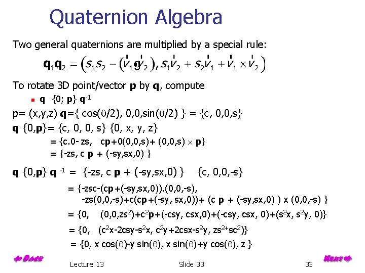
Quaternion Algebra Two general quaternions are multiplied by a special rule: To rotate 3 D point/vector p by q, compute n q {0; p} q-1 p= (x, y, z) q={ cos(q/2), 0, 0, sin(q/2) } = {c, 0, 0, s} q {0, p}= {c, 0, 0, s} {0, x, y, z} = {c. 0 - zs, cp+0(0, 0, s)+ (0, 0, s) p} = {-zs, c p + (-sy, sx, 0) } q {0, p} q -1 = {-zs, c p + (-sy, sx, 0) } {c, 0, 0, -s} = {-zsc-(cp+(-sy, sx, 0)). (0, 0, -s), -zs(0, 0, -s)+c(cp+(-sy, sx, 0))+ (c p + (-sy, sx, 0) ) x (0, 0, -s) } = {0, (0, 0, zs 2)+c 2 p+(-csy, csx, 0)+(s 2 x, s 2 y, 0)} = {0, (c 2 x-2 csy-s 2 x, c 2 y+2 csx-s 2 y, zs 2+sc 2)} = {0, x cos(q)-y sin(q), x sin(q)+y cos(q), z } Lecture 13 Slide 33 33

Quaternion Algebra Two general quaternions are multiplied by a special rule: To rotate 3 D point/vector p by q, compute n q {0; p} q-1 Quaternions are associative: n (q 1 q 2) q 3 = q 1 (q 2 q 3) But not commutative: n q 1 q 2 q 1 Lecture 13 Slide 34 34

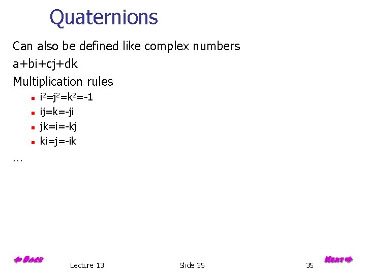
Quaternions Can also be defined like complex numbers a+bi+cj+dk Multiplication rules n n i 2=j 2=k 2=-1 ij=k=-ji jk=i=-kj ki=j=-ik … Lecture 13 Slide 35 35

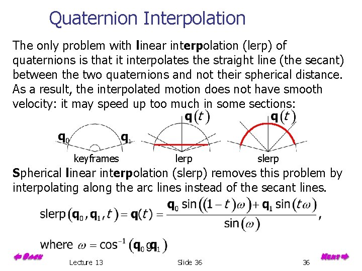
Quaternion Interpolation The only problem with linear interpolation (lerp) of quaternions is that it interpolates the straight line (the secant) between the two quaternions and not their spherical distance. As a result, the interpolated motion does not have smooth velocity: it may speed up too much in some sections: keyframes lerp slerp Spherical linear interpolation (slerp) removes this problem by interpolating along the arc lines instead of the secant lines. Lecture 13 Slide 36 36

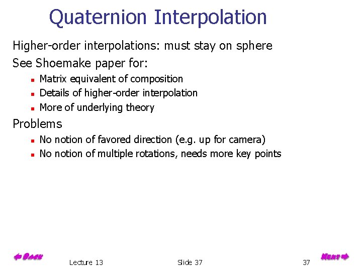
Quaternion Interpolation Higher-order interpolations: must stay on sphere See Shoemake paper for: n n n Matrix equivalent of composition Details of higher-order interpolation More of underlying theory Problems n n No notion of favored direction (e. g. up for camera) No notion of multiple rotations, needs more key points Lecture 13 Slide 37 37

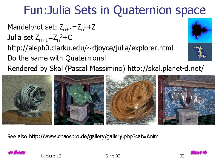
Fun: Julia Sets in Quaternion space Mandelbrot set: Zn+1=Zn 2+Z 0 Julia set Zn+1=Zn 2+C http: //aleph 0. clarku. edu/~djoyce/julia/explorer. html Do the same with Quaternions! Rendered by Skal (Pascal Massimino) http: //skal. planet-d. net/ See also http: //www. chaospro. de/gallery. php? cat=Anim Lecture 13 Slide 38 38

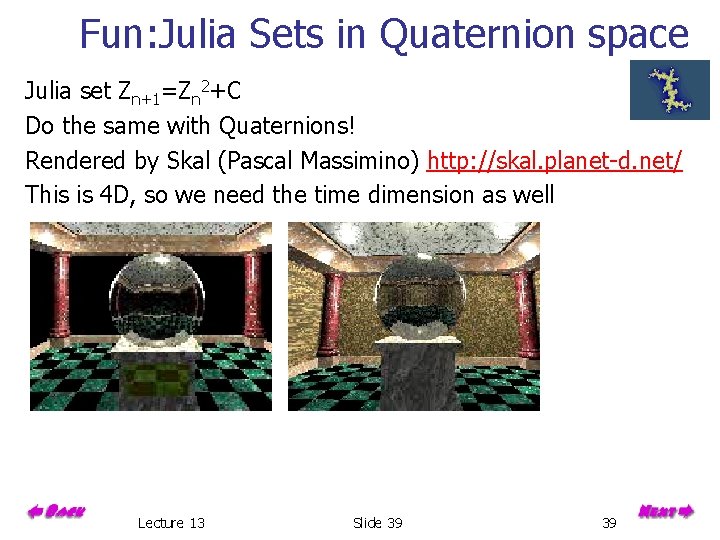
Fun: Julia Sets in Quaternion space Julia set Zn+1=Zn 2+C Do the same with Quaternions! Rendered by Skal (Pascal Massimino) http: //skal. planet-d. net/ This is 4 D, so we need the time dimension as well Lecture 13 Slide 39 39

Overview Keyframing and interpolation Interpolation of rotations, quaternions Kimematrics, articulation Physisally-based simulation & particles Lecture 13 Slide 40 40

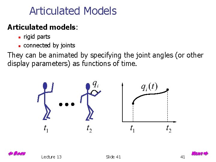
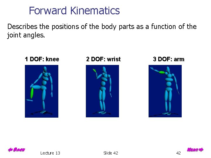
Articulated Models Articulated models: n n rigid parts connected by joints They can be animated by specifying the joint angles (or other display parameters) as functions of time. Lecture 13 Slide 41 41

Forward Kinematics Describes the positions of the body parts as a function of the joint angles. 1 DOF: knee Lecture 13 2 DOF: wrist Slide 42 3 DOF: arm 42

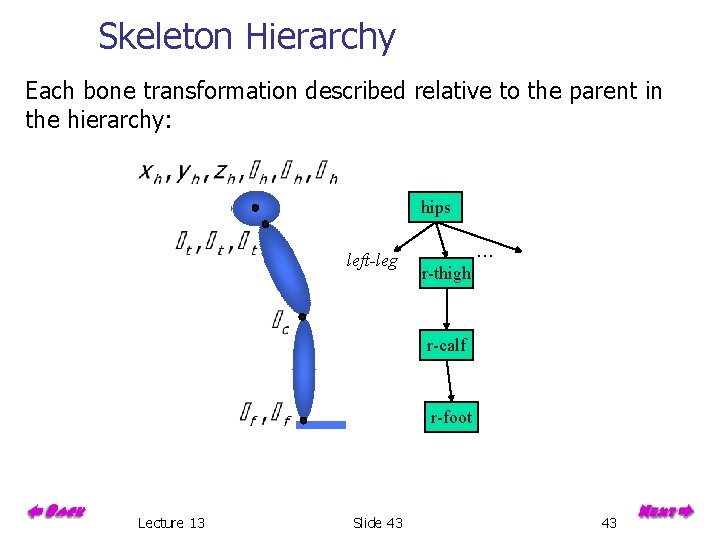
Skeleton Hierarchy Each bone transformation described relative to the parent in the hierarchy: hips left-leg . . . r-thigh r-calf r-foot Lecture 13 Slide 43 43

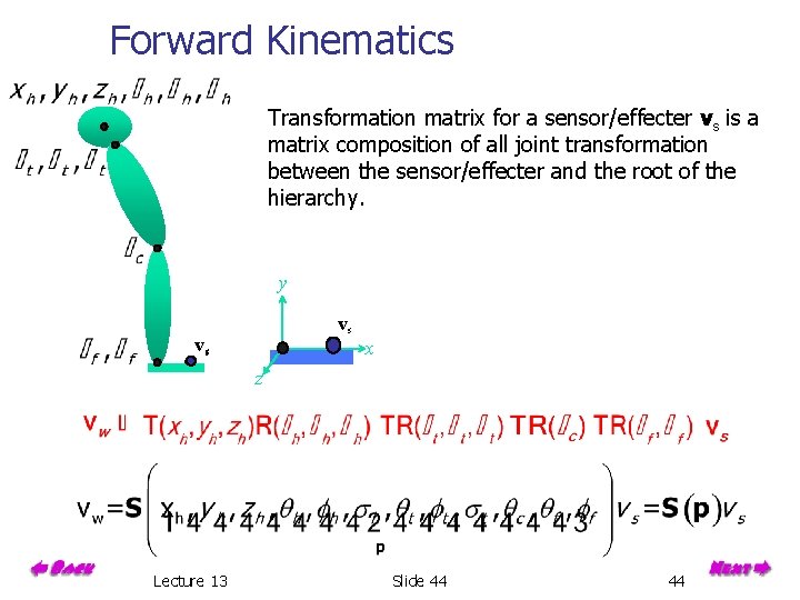
Forward Kinematics Transformation matrix for a sensor/effecter vs is a matrix composition of all joint transformation between the sensor/effecter and the root of the hierarchy. y vs vs x z Lecture 13 Slide 44 44

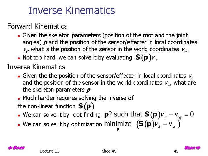
Inverse Kinematics Forward Kinematics n n Given the skeleton parameters (position of the root and the joint angles) p and the position of the sensor/effecter in local coordinates vs, what is the position of the sensor in the world coordinates vw. Not too hard, we can solve it by evaluating Inverse Kinematics Given the position of the sensor/effecter in local coordinates vs and the position of the sensor in the world coordinates vw, what are the skeleton parameters p. n Much harder requires solving the inverse of the non-linear function n We can solve it by root-finding n n We can solve it by optimization Lecture 13 Slide 45 45

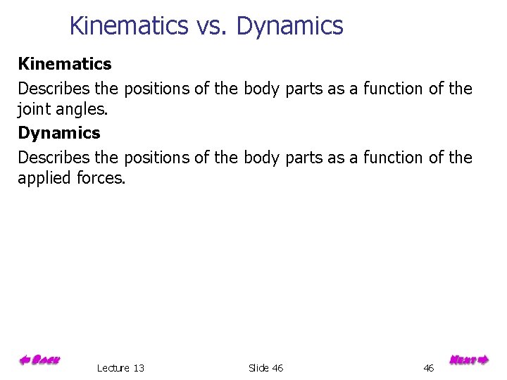
Kinematics vs. Dynamics Kinematics Describes the positions of the body parts as a function of the joint angles. Dynamics Describes the positions of the body parts as a function of the applied forces. Lecture 13 Slide 46 46

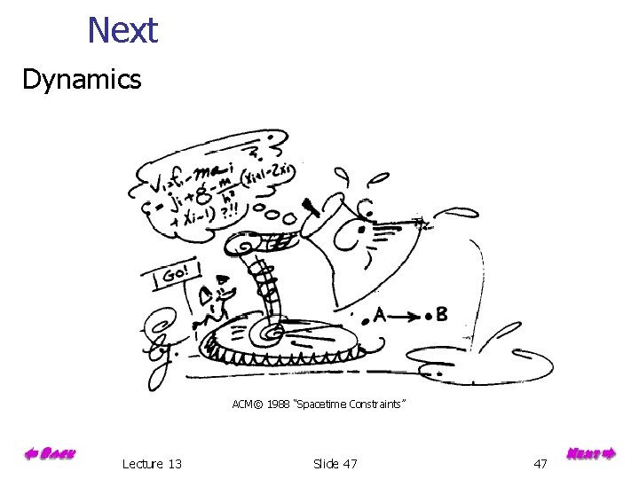
Next Dynamics ACM© 1988 “Spacetime Constraints” Lecture 13 Slide 47 47

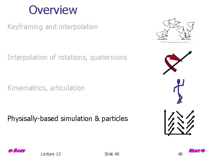
Overview Keyframing and interpolation Interpolation of rotations, quaternions Kimematrics, articulation Physisally-based simulation & particles Lecture 13 Slide 48 48

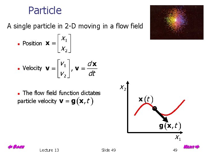
Particle A single particle in 2 -D moving in a flow field n Position n Velocity The flow field function dictates particle velocity n Lecture 13 Slide 49 49

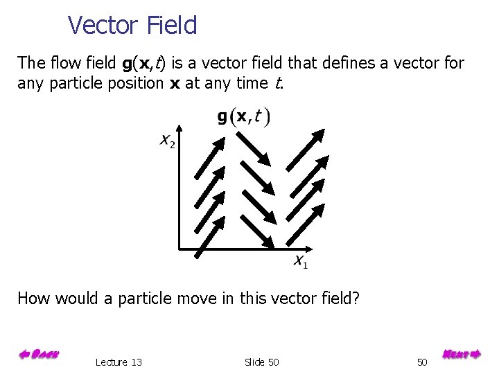
Vector Field The flow field g(x, t) is a vector field that defines a vector for any particle position x at any time t. How would a particle move in this vector field? Lecture 13 Slide 50 50

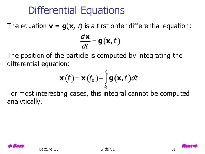
Differential Equations The equation v = g(x, t) is a first order differential equation: The position of the particle is computed by integrating the differential equation: For most interesting cases, this integral cannot be computed analytically. Lecture 13 Slide 51 51

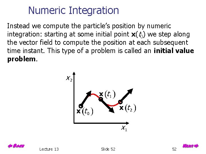
Numeric Integration Instead we compute the particle’s position by numeric integration: starting at some initial point x(t 0) we step along the vector field to compute the position at each subsequent time instant. This type of a problem is called an initial value problem. Lecture 13 Slide 52 52

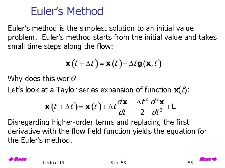
Euler’s Method Euler’s method is the simplest solution to an initial value problem. Euler’s method starts from the initial value and takes small time steps along the flow: Why does this work? Let’s look at a Taylor series expansion of function x(t): Disregarding higher-order terms and replacing the first derivative with the flow field function yields the equation for the Euler’s method. Lecture 13 Slide 53 53

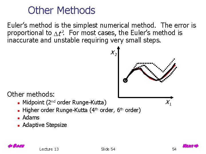
Other Methods Euler’s method is the simplest numerical method. The error is proportional to. For most cases, the Euler’s method is inaccurate and unstable requiring very small steps. Other methods: n n Midpoint (2 nd order Runge-Kutta) Higher order Runge-Kutta (4 th order, 6 th order) Adams Adaptive Stepsize Lecture 13 Slide 54 54

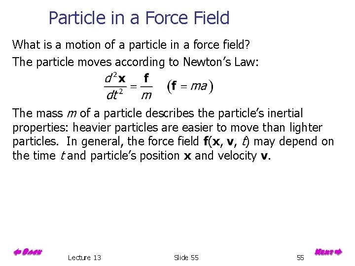
Particle in a Force Field What is a motion of a particle in a force field? The particle moves according to Newton’s Law: The mass m of a particle describes the particle’s inertial properties: heavier particles are easier to move than lighter particles. In general, the force field f(x, v, t) may depend on the time t and particle’s position x and velocity v. Lecture 13 Slide 55 55

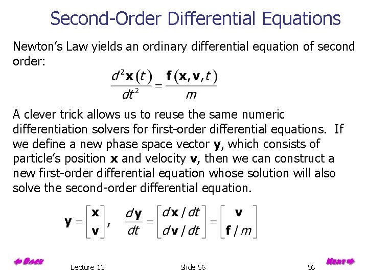
Second-Order Differential Equations Newton’s Law yields an ordinary differential equation of second order: A clever trick allows us to reuse the same numeric differentiation solvers for first-order differential equations. If we define a new phase space vector y, which consists of particle’s position x and velocity v, then we can construct a new first-order differential equation whose solution will also solve the second-order differential equation. Lecture 13 Slide 56 56

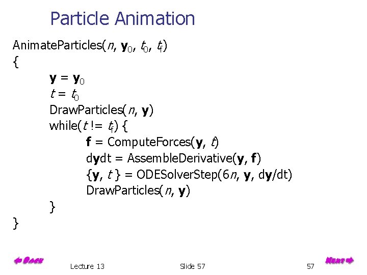
Particle Animation Animate. Particles(n, y 0, tf) { y = y 0 t = t 0 Draw. Particles(n, y) while(t != tf) { f = Compute. Forces(y, t) dydt = Assemble. Derivative(y, f) {y, t } = ODESolver. Step(6 n, y, dy/dt) Draw. Particles(n, y) } } Lecture 13 Slide 57 57

Particle Animation [Reeves et al. 1983] Start Trek, The Wrath of Kahn Star Trek, The Wrath of Kahn [Reeves et al. 1983] Lecture 13 Slide 58 58

Particle Modeling Lecture 13 [Reeves et al. 1983] Slide 59 59

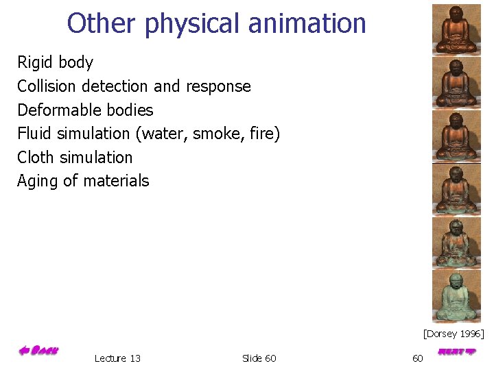
Other physical animation Rigid body Collision detection and response Deformable bodies Fluid simulation (water, smoke, fire) Cloth simulation Aging of materials [Dorsey 1996] Lecture 13 Slide 60 60

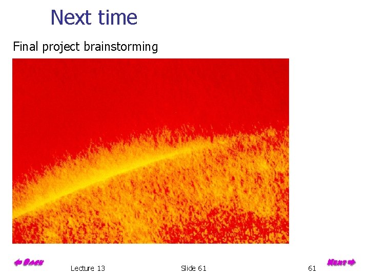
Next time Final project brainstorming Lecture 13 Slide 61 61