Anderson Localization for the Nonlinear Schrdinger Equation NLSE

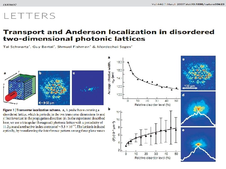
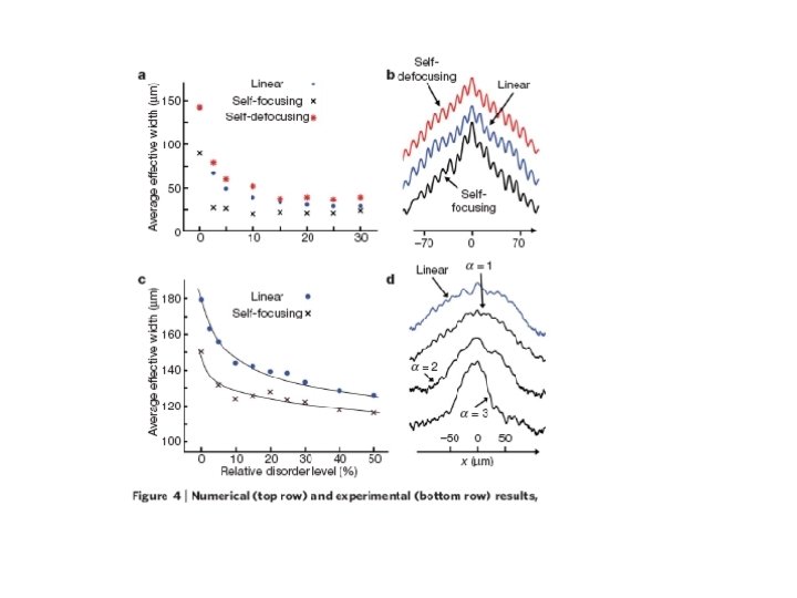
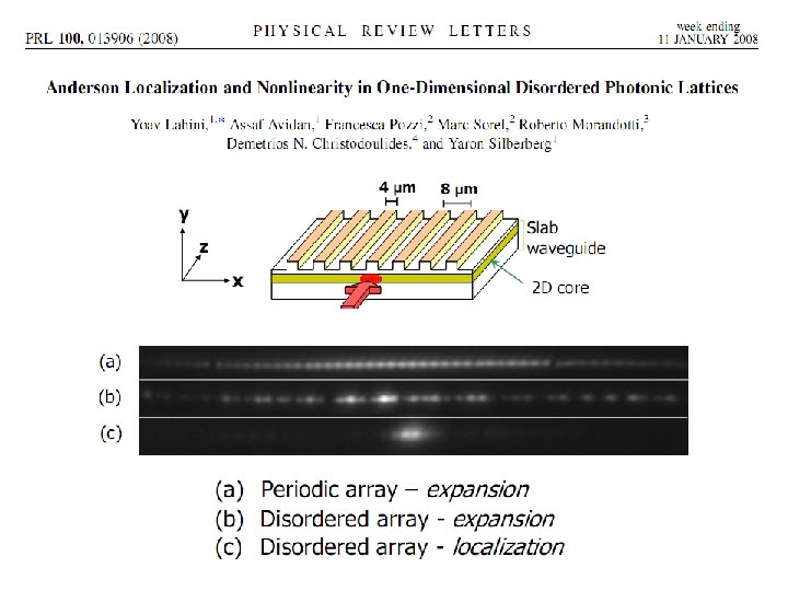
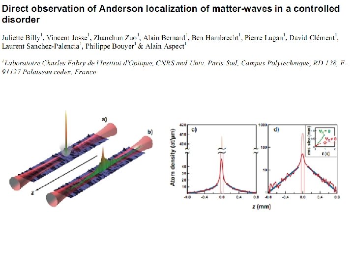
Anderson Localization for the Nonlinear Schrödinger Equation (NLSE): Results and Puzzles Yevgeny Krivolapov, Hagar Veksler, Avy Soffer, and SF Experimental Relevance Nonlinear Optics Bose Einstein Condensates (BECs) Competition between randomness and nonlinearity

The Nonlinear Schroedinger (NLS) Equation 1 D lattice version 1 D continuum version random Anderson Model

localization Does Localization Survive the Nonlinearity? ? ? Work in progress, several open questions Aim: find a clear estimate, at least for a finite (long) time

Does Localization Survive the Nonlinearity? ? ? • Yes, if there is spreading the magnitude of the nonlinear term decreases and localization takes over. • No, assume wave-packet width is then the relevant energy spacing is , the perturbation because of the nonlinear term is and all depends on • No, but does not depend on • No, but it depends on realizations • Yes, because some time dependent quasiperiodic localized perturbation does not destroy localization

Does Localization Survive the Nonlinearity? • No, the NLSE is a chaotic dynamical system. • No, but localization asymptotically preserved beyond some front that is logarithmic in time

Numerical Simulations • In regimes relevant for experiments looks that localization takes place • Spreading for long time (Shepelyansky, Pikovsky, Molina, Kopidakis, Komineas, Flach, Aubry) • We do not know the relevant space and time scales • All results in Split-Step • No control (but may be correct in some range) • Supported by various heuristic arguments

Pikovsky, Sheplyansky

Pikovsky, Shepelyansky S. Flach, D. Krimer and S. Skokos t b, g, r 0. 1, 1, 5

Modified NLSE H. Veksler, Y. Krivolapov, SF Shepelyansky-Pikovsky arguments –No spreading for Flach, Krimer and Sokos for

p= 1. 5, 2, 2. 5, 4, 8, 0 (top to bottom) Also M. Mulansky

Heuristic Theories that Involve Noise Assumptions Clearly Contradict Numerical Results: 1. Nothing happens at 2. approach to localization at These theories may have a range of validity

Perturbation Theory The nonlinear Schroedinger Equation on a Lattice in 1 D random Eigenstates Anderson Model

The states are indexed by their centers of localization Is a state localized near realization for realizations of measure This is possible since nearly each state has a Localization center and in a box size M there approximately M states Indexing by “center of mass” more stable

Overlap of the range of the localization length perturbation expansion Iterative calculation of start at

start at Step 1 Secular term to be removed by here

Secular terms can be removed in all orders by New ansatz The problem of small denominators The Aizenman-Molchanov approach (fractional moments)

Step 2

Secular term removed

To different realization

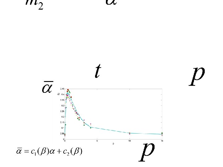
Second order Red=perturbative, blue=exact

Third order

Second order Blue=exact, red=linear Third order

Second order

Aim: to use perturbation theory to obtain a numerical solution that is controlled aposteriory

General removal of secular terms Remove secular terms In order k with

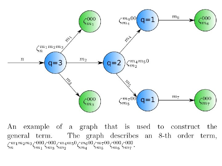
Number of terms in higher orders iterate number of products of in places subtract forbidden combinations

The solid line denotes the exact numerical solution of the recurrence relation for and dashed line is the asymptotic upper bound on this solution

Bounding the General Term results in products of the form

Using Cauchy-Schwartz inequality

Small denominators If the shape of the squares of the eigenfunctions sufficiently different, using a recent result of Aizenman and Warzel we propose

Assuming sufficient independence between states localized far away

Chebychev inequality

Bound on products Average over realizations of measure and with the help of the generalized Hoelder inequality continue to longer products for example

Bound on general term The Bound deteriorates with order

The remainder Bound by a bootstrap argument

The Bound on the remainder One can show that for strong disorder It is probably proportional to Front logarithmic in time and the constant are multiplied by

Bound on error • Solve linear equation for the remainder of order • If bounded to time perturbation theory accurate to that time (numerics) • Order of magnitude estimate if asymptotic hence for optimal order (up to constants).

Perturbation theory steps • • • Expansion in nonlinearity Removal of secular terms Control of denominators Probabilistic bound on general term Control of remainder

Summary 1. 2. 3. 4. 5. 6. 7. 8. A perturbation expansion in was developed Secular terms were removed A bound on the general term was derived Results were tested numerically A bound on the remainder was obtained, indicating that the series is asymptotic. For limited time tending to infinity for small nonlinearity, front logarithmic in time or Improved for strong disorder Earlier result: exponential localization for times shorter than

Open problems 1. Can the logarithmic front be found for arbitrary long time? 2. Is the series asymptotic or convergent? Under what conditions? Can the series be resummed? Can the bound on the general term be improved? Rigorous proof of the various conjectures on the linear, Anderson model 3. 4. 5. 6. How to use to produce an aposteriory bound?