Analyzing TwoVariable Data Lesson 2 5 2 6

Analyzing Two-Variable Data Lesson 2. 5 & 2. 6 Regression Lines Statistics and Probability with Applications, 3 rd Edition Starnes & Tabor Bedford Freeman Worth Publishers

The Least-Squares Regression Line Learning Targets After this lesson, you should be able to: ü Calculate the equation of the least-squares regression line using technology. ü Calculate the equation of the least-squares regression line using summary statistics. ü Describe how outliers affect the least-squares regression line. ü Make predictions using regression lines, keeping in mind the dangers of extrapolation. ü Calculate and interpret a residual. ü Interpret the slope and y intercept of a regression line. Statistics and Probability with Applications, 3 rd Edition 2

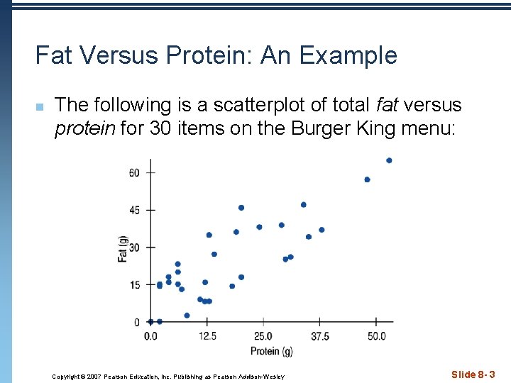
Fat Versus Protein: An Example n The following is a scatterplot of total fat versus protein for 30 items on the Burger King menu: Copyright © 2007 Pearson Education, Inc. Publishing as Pearson Addison-Wesley Slide 8 - 3

The Linear Model n n n Correlation says “There seems to be a linear association between these two variables, ” but it doesn’t tell what that association is. We can say more about the linear relationship between two quantitative variables with a model. A model simplifies reality to help us understand underlying patterns and relationships. Copyright © 2007 Pearson Education, Inc. Publishing as Pearson Addison-Wesley Slide 8 - 4

The Linear Model (cont. ) n The linear model is just an equation of a straight line through the data. n The points in the scatterplot don’t all line up, but a straight line can summarize the general pattern. n The linear model can help us understand how the values are associated. Copyright © 2007 Pearson Education, Inc. Publishing as Pearson Addison-Wesley Slide 8 - 5

Residuals n n n The model won’t be perfect, regardless of the line we draw. Some points will be above the line and some will be below. The estimate made from a model is the predicted value (denoted as ). Copyright © 2007 Pearson Education, Inc. Publishing as Pearson Addison-Wesley Slide 8 - 6

Residuals (cont. ) n n The difference between the observed value and its associated predicted value is called the residual. To find the residuals, we always subtract the predicted value from the observed one: Copyright © 2007 Pearson Education, Inc. Publishing as Pearson Addison-Wesley Slide 8 - 7

Residuals (cont. ) n n A negative residual means the predicted value’s too big (an overestimate). A positive residual means the predicted value’s too small (an underestimate). Copyright © 2007 Pearson Education, Inc. Publishing as Pearson Addison-Wesley Slide 8 - 8

“Best Fit” Means Least Squares n n n Some residuals are positive, others are negative, and, on average, they cancel each other out. So, we can’t assess how well the line fits by adding up all the residuals. Similar to what we did with deviations, we square the residuals and add the squares. The smaller the sum, the better the fit. The line of best fit is the line for which the sum of the squared residuals is smallest. Copyright © 2007 Pearson Education, Inc. Publishing as Pearson Addison-Wesley Slide 8 - 9

Least Squares Regression Line LSRL • The line that gives the best fit to the data set • The line that minimizes the sum of the squares of the deviations from the line

(3, 10) y =. 5(6) + 4 = 7 4. 5 2 – 7 = -5 y =. 5(0) + 4 = 4 0 – 4 = -4 y =. 5(3) + 4 = 5. 5 -4 (0, 0) 10 – 5. 5 = 4. 5 -5 (6, 2) Sum of the squares = 61. 25

What is the sum of the deviations from the line? Will it always be zero? (3, 10) Use a calculator to find the line of best fit 6 Find y - y The line that minimizes the sum of the squares of the deviations from the line -3 is the LSRL (0, 0) -3 (6, 2) Sum of the squares = 54

HOW TO USE THE CALCULATOR TO FIND LSRL • Enter your data in L 1 and L 2. (Note: Be sure that your Stat Plot is on and indicates the Lists you are using. ) • Go to [STAT] "CALC" "8: Lin. Reg(a+bx). This is the LSRL. • Enter L 1, L 2, Y 1 OR JUST “ENTER” IF YOU HAVE AN OLDER CALCULATOR • To view, go to [Zoom] "9: Zoom. Stat". Slide 7 - 13

Least Squares Regression Line LSRL You may see the equation written in the form: - (y-hat) means the predicted y n Be sure to put the hat on the y Copyright © 2007 Pearson Education, Inc. Publishing as Pearson Addison-Wesley

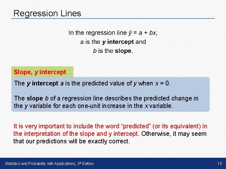
Regression Lines Slope, y intercept The y intercept a is the predicted value of y when x = 0. The slope b of a regression line describes the predicted change in the y variable for each one-unit increase in the x variable. It is very important to include the word “predicted” (or its equivalent) in the interpretation of the slope and y intercept. Otherwise, it may seem that our predictions will be exactly correct. Statistics and Probability with Applications, 3 rd Edition 15

The ages (in months) and heights (in inches) of seven children are given. x 16 24 42 60 75 102 120 y 24 30 35 40 48 56 60 Find the LSRL. Interpret the slope and y-intercept in the context of the problem. Copyright © 2007 Pearson Education, Inc. Publishing as Pearson Addison-Wesley

Slope: For an increase in age of one month, month there is an approximate increase of. 34 inches in heights of children. Y-Intercept: the predicted height of a newborn is 20 inches Copyright © 2007 Pearson Education, Inc. Publishing as Pearson Addison-Wesley

The ages (in months) and heights (in inches) of seven children are given. x 16 24 42 60 75 102 120 y 24 30 35 40 48 56 60 Predict the height of a child who is 4. 5 years old. Predict the height of someone who is 20 years old. Copyright © 2007 Pearson Education, Inc. Publishing as Pearson Addison-Wesley

Interpretations SPLOPE is a rate of change and it explains how an increase in the explanatory variable affects the response. Y-INTERCEPT shows you what's predicted for the response when the explanatory value is zero, and sometimes it doesn't have a meaningful interpretation. Doesn't mean we shouldn't know how to interpret it, just sometimes it doesn't make a whole lot of sense in context. Sometimes it falls outside that reasonable predictions window. Statistics and Probability with Applications, 3 rd Edition 19

Fat Versus Protein: An Example • The regression line for the Burger King data fits the data well: – The equation is – Find and interpret slope & yintercept – Using the equation for our line we can predict the fat content for a 30 g of protein BK Broiler chicken sandwich as: 6. 8 + 0. 97(30) = 35. 9 grams of fat. Note that the actual fat content is about 25 g. Statistics and Probability with Applications, 3 rd Edition Slide 8 - 2020

Regression Lines Given the graph below, can we predict the price of a Ford F-150 with 300, 000 miles driven? We can certainly substitute 300, 000 into the equation of the line. The prediction is yˆ = 38, 257 − 0. 1629(300, 000) = −$10, 613 This prediction is an extrapolation. Extrapolation is the use of a regression line for prediction far outside the interval of x values used to obtain the line. Such predictions are often not accurate. Statistics and Probability with Applications, 3 rd Edition 21

Extrapolation: Reaching Beyond the Data • Linear models give a predicted value for each case in the data. • We cannot assume that a linear relationship in the data exists beyond the range of the data. • Once we venture into new x territory, such a prediction is called an extrapolation. • The LSRL should not be used to predict y for values of x outside the data set. Statistics and Probability with Applications, 3 rd Edition 22

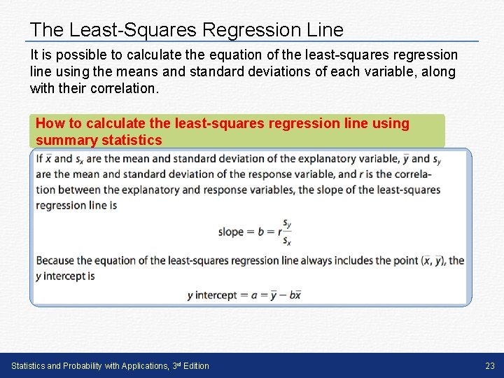
The Least-Squares Regression Line It is possible to calculate the equation of the least-squares regression line using the means and standard deviations of each variable, along with their correlation. How to calculate the least-squares regression line using summary statistics Statistics and Probability with Applications, 3 rd Edition 23

The following statistics are found for the variables posted speed limit and the average number of accidents. Find the LSRL & predict the number of accidents for a posted speed limit of 50 mph. Copyright © 2007 Pearson Education, Inc. Publishing as Pearson Addison-Wesley

Computer Regression Output Least-Squares Regression A number of statistical software packages produce similar regression output. Be sure you can locate n the slope b, n the y intercept a, n and the values of s and r 2. + n Interpreting

Computer-generated regression analysis of knee surgery Be sure to convert r 2 data: NEVER use to decimal before 2 adjusted r ! taking the square Predictor Coef Stdev T P root! Constant 107. 58 What is 11. 12 9. 67 of 0. 000 the equation the is the correlation Age What 0. 8710 0. 4146 LSRL? 2. 10 0. 062 coefficient? Find the slope & y-intercept. s = 10. 42 R-sq = 30. 6% Copyright © 2007 Pearson Education, Inc. Publishing as Pearson Addison-Wesley R-sq(adj) = 23. 7%

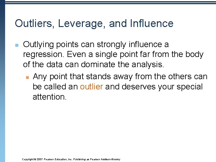
Outliers, Leverage, and Influence n Outlying points can strongly influence a regression. Even a single point far from the body of the data can dominate the analysis. n Any point that stands away from the others can be called an outlier and deserves your special attention. Copyright © 2007 Pearson Education, Inc. Publishing as Pearson Addison-Wesley

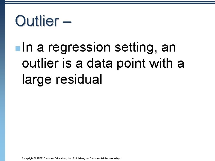
Outlier – n In a regression setting, an outlier is a data point with a large residual Copyright © 2007 Pearson Education, Inc. Publishing as Pearson Addison-Wesley

Influential point. A point that influences where the LSRL is located n If removed, it will significantly change the slope of the LSRL n Copyright © 2007 Pearson Education, Inc. Publishing as Pearson Addison-Wesley

Outliers, Leverage, and Influence (cont. ) n The following scatterplot shows that something was awry in Palm Beach County, Florida, during the 2000 presidential election… Copyright © 2007 Pearson Education, Inc. Publishing as Pearson Addison-Wesley

Outliers, Leverage, and Influence (cont. ) n The red line shows the effects that one unusual point can have on a regression: Copyright © 2007 Pearson Education, Inc. Publishing as Pearson Addison-Wesley

Outliers, Leverage, and Influence (cont. ) n n The linear model doesn’t fit points with large residuals very well. Because they seem to be different from the other cases, it is important to pay special attention to points with large residuals. Copyright © 2007 Pearson Education, Inc. Publishing as Pearson Addison-Wesley

Lurking Variables and Causation n n No matter how strong the association, no matter how straight the line, there is no way to conclude from a regression alone that one variable causes the other. n There’s always the possibility that some third variable is driving both of the variables you have observed. With observational data, as opposed to data from a designed experiment, there is no way to be sure that a lurking variable is not the cause of any apparent association. Copyright © 2007 Pearson Education, Inc. Publishing as Pearson Addison-Wesley

Lurking Variables and Causation (cont. ) n The following scatterplot shows that the average life expectancy for a country is related to the number of doctors person in that country: Copyright © 2007 Pearson Education, Inc. Publishing as Pearson Addison-Wesley

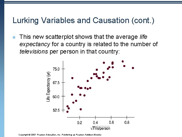
Lurking Variables and Causation (cont. ) n This new scatterplot shows that the average life expectancy for a country is related to the number of televisions person in that country: Copyright © 2007 Pearson Education, Inc. Publishing as Pearson Addison-Wesley

Lurking Variables and Causation (cont. ) n n Since televisions are cheaper than doctors, send TVs to countries with low life expectancies in order to extend lifetimes. Right? How about considering a lurking variable? That makes more sense… n Countries with higher standards of living have both longer life expectancies and more doctors (and TVs!). n If higher living standards cause changes in these other variables, improving living standards might be expected to prolong lives and increase the numbers of doctors and TVs. Copyright © 2007 Pearson Education, Inc. Publishing as Pearson Addison-Wesley