Analyzing OneVariable Data Lesson 1 9 Describing Location

Analyzing One-Variable Data Lesson 1. 9 Describing Location in a Distribution Statistics and Probability with Applications, 3 rd Edition Starnes, Tabor Bedford Freeman Worth Publishers

Describing Location in a Distribution Learning Targets After this lesson, you should be able to: ü Find and interpret a percentile in a distribution of quantitative data. ü Estimate percentiles and individual values using a cumulative relative frequency graph. ü Find and interpret a standardized score (z-score) in a distribution of quantitative data. Statistics and Probability with Applications, 3 rd Edition 2

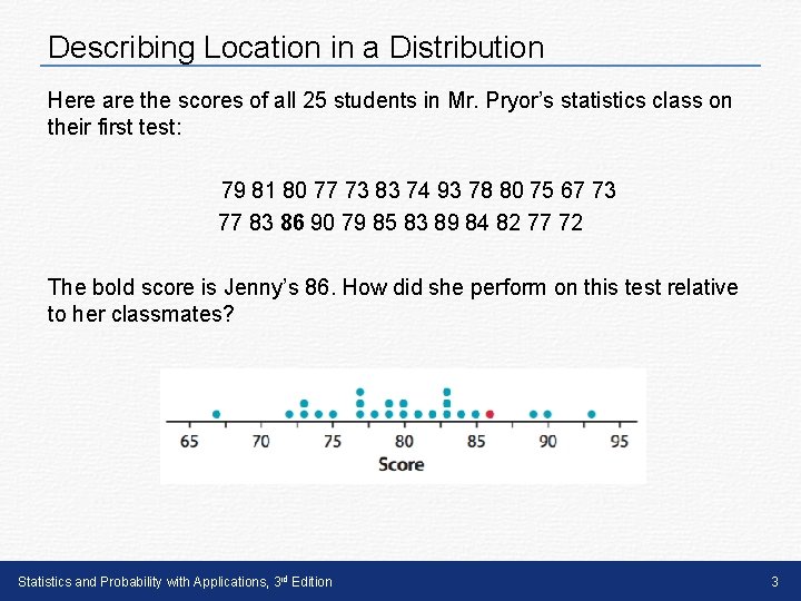
Describing Location in a Distribution Here are the scores of all 25 students in Mr. Pryor’s statistics class on their first test: 79 81 80 77 73 83 74 93 78 80 75 67 73 77 83 86 90 79 85 83 89 84 82 77 72 The bold score is Jenny’s 86. How did she perform on this test relative to her classmates? Statistics and Probability with Applications, 3 rd Edition 3

Describing Location in a Distribution One way to describe Jenny’s location in the distribution of test scores is to calculate her percentile. Percentile An individual’s percentile is the percent of values in a distribution that are less than the individual’s data value. Because 21 of the 25 observations (84%) are below her score, Jenny is at the 84 th percentile in the class’s test score distribution. Be careful with your language when describing percentiles. Percentiles are specific locations in a distribution, so an observation isn’t “in” the 84 th percentile. Rather, it is “at” the 84 th percentile. Statistics and Probability with Applications, 3 rd Edition 4

Describing Location in a Distribution There are some interesting graphs that can be made with percentiles. One of the most common starts with a frequency table for a quantitative variable and expands it to include cumulative frequency and cumulative relative frequency. Cumulative Relative Frequency Graph A cumulative relative frequency graph plots a point corresponding to the cumulative relative frequency in each interval at the smallest value of the next interval, starting with a point at a height of 0% at the smallest value of the first interval. Consecutive points are then connected with a line segment to form the graph. Statistics and Probability with Applications, 3 rd Edition 5

+ • Cumulative Relative Frequency Graphs Age Frequency Relative frequency Cumulative relative frequency 40 -44 2 2/44 = 4. 5% 45 -49 7 7/44 = 15. 9% 9 9/44 = 20. 5% 50 -54 13 13/44 = 29. 5% 22 22/44 = 50. 0% 55 -59 12 12/44 = 34% 34 34/44 = 77. 3% 60 -64 7 7/44 = 15. 9% 41 41/44 = 93. 2% 65 -69 3 3/44 = 6. 8% 44 44/44 = 100% Describing Location in a Distribution Age of First 44 Presidents When They Were Inaugurated

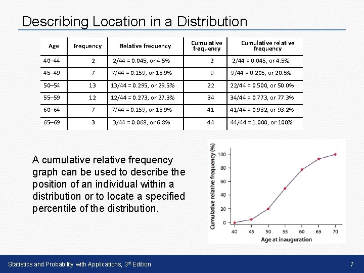
Describing Location in a Distribution Age Frequency Relative frequency Cumulative relative frequency 40– 44 2 2/44 = 0. 045, or 4. 5% 45– 49 7 7/44 = 0. 159, or 15. 9% 9 9/44 = 0. 205, or 20. 5% 50– 54 13 13/44 = 0. 295, or 29. 5% 22 22/44 = 0. 500, or 50. 0% 55– 59 12 12/44 = 0. 273, or 27. 3% 34 34/44 = 0. 773, or 77. 3% 60– 64 7 7/44 = 0. 159, or 15. 9% 41 41/44 = 0. 932, or 93. 2% 65– 69 3 3/44 = 0. 068, or 6. 8% 44 44/44 = 1. 000, or 100% A cumulative relative frequency graph can be used to describe the position of an individual within a distribution or to locate a specified percentile of the distribution. Statistics and Probability with Applications, 3 rd Edition 7

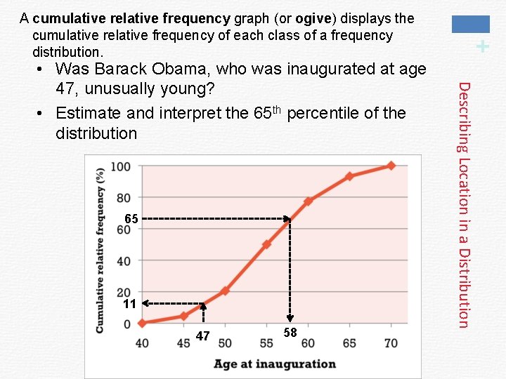
65 11 47 58 Describing Location in a Distribution • Was Barack Obama, who was inaugurated at age 47, unusually young? • Estimate and interpret the 65 th percentile of the distribution + A cumulative relative frequency graph (or ogive) displays the cumulative relative frequency of each class of a frequency distribution.

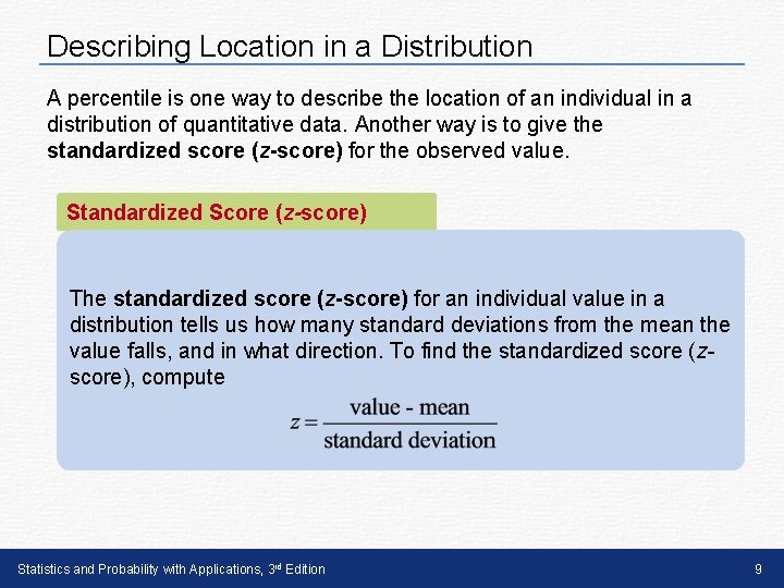
Describing Location in a Distribution A percentile is one way to describe the location of an individual in a distribution of quantitative data. Another way is to give the standardized score (z-score) for the observed value. Standardized Score (z-score) The standardized score (z-score) for an individual value in a distribution tells us how many standard deviations from the mean the value falls, and in what direction. To find the standardized score (zscore), compute Statistics and Probability with Applications, 3 rd Edition 9

The Standard Deviation as a Ruler • The trick in comparing very different-looking values is to use standard deviations as our rulers. • The standard deviation tells us how the whole collection of values varies, so it’s a natural ruler for comparing an individual to a group. • As the most common measure of variation, the standard deviation plays a crucial role in how we look at data. Slide 6 -and 10 Probability with Applications, 3 rd Edition Statistics 10

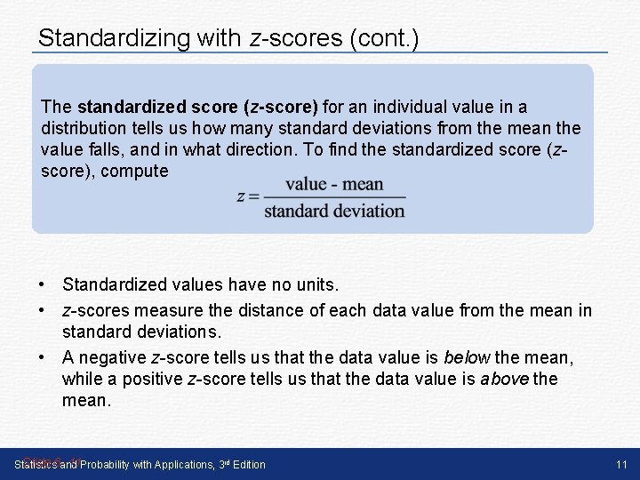
Standardizing with z-scores (cont. ) The standardized score (z-score) for an individual value in a distribution tells us how many standard deviations from the mean the value falls, and in what direction. To find the standardized score (zscore), compute • Standardized values have no units. • z-scores measure the distance of each data value from the mean in standard deviations. • A negative z-score tells us that the data value is below the mean, while a positive z-score tells us that the data value is above the mean. Slide 6 -and 11 Probability with Applications, 3 rd Edition Statistics 11

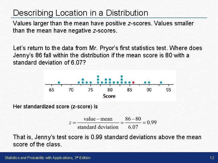
Describing Location in a Distribution Values larger than the mean have positive z-scores. Values smaller than the mean have negative z-scores. Let’s return to the data from Mr. Pryor’s first statistics test. Where does Jenny’s 86 fall within the distribution if the mean score is 80 with a standard deviation of 6. 07? Her standardized score (z-score) is That is, Jenny’s test score is 0. 99 standard deviations above the mean score of the class. Statistics and Probability with Applications, 3 rd Edition 12

Benefits of Standardizing • Standardized values have been converted from their original units to the standard statistical unit of standard deviations from the mean. • Thus, we can compare values that are measured on different scales, with different units, or from different populations. • A z-score gives us an indication of how unusual a value is because it tells us how far it is from the mean. • Remember that a negative z-score tells us that the data value is below the mean, while a positive z-score tells us that the data value is above the mean. • The larger a z-score is (negative or positive), the more unusual it is. Slide 6 -and 13 Probability with Applications, 3 rd Edition Statistics 13

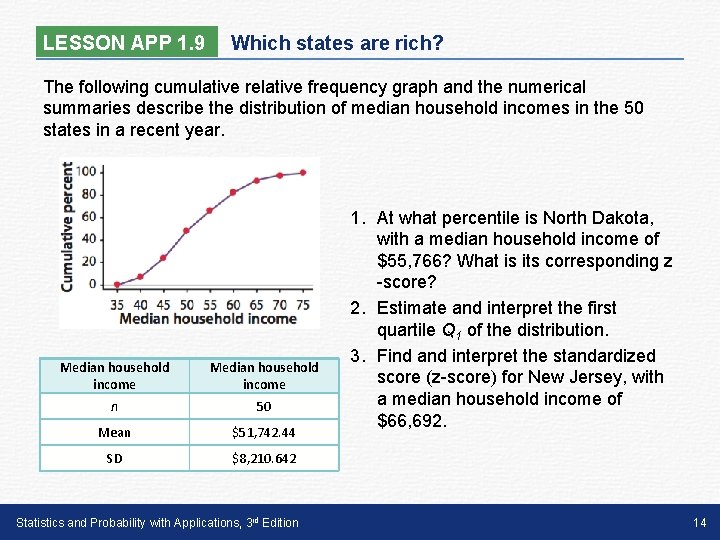
LESSON APP 1. 9 Which states are rich? The following cumulative relative frequency graph and the numerical summaries describe the distribution of median household incomes in the 50 states in a recent year. Median household income n 50 Mean $51, 742. 44 SD $8, 210. 642 Statistics and Probability with Applications, 3 rd Edition 1. At what percentile is North Dakota, with a median household income of $55, 766? What is its corresponding z -score? 2. Estimate and interpret the first quartile Q 1 of the distribution. 3. Find and interpret the standardized score (z-score) for New Jersey, with a median household income of $66, 692. 14

Describing Location in a Distribution Learning Targets After this lesson, you should be able to: ü Find and interpret a percentile in a distribution of quantitative data. ü Estimate percentiles and individual values using a cumulative relative frequency graph. ü Find and interpret a standardized score (z-score) in a distribution of quantitative data. Statistics and Probability with Applications, 3 rd Edition 15