Analyzing Mixed Costs APPENDIX 5 A Power Point

Analyzing Mixed Costs APPENDIX 5 A Power. Point Authors: Susan Coomer Galbreath, Ph. D. , CPA Jon A. Booker, Ph. D. , CPA, CIA Cynthia J. Rooney, Ph. D. , CPA ©Mc. Graw-Hill Education. All rights reserved. Authorized only for instructor use in the classroom. No reproduction or fur distribution permitted without the prior written consent of Mc. Graw-Hill Education.

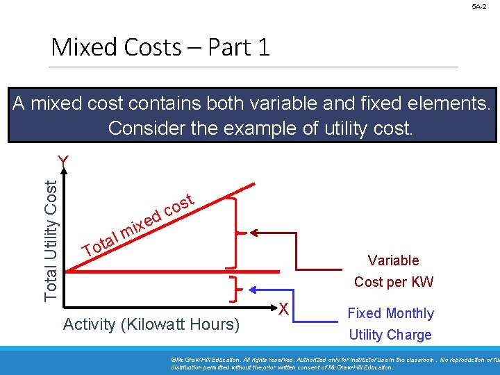
5 A-2 Mixed Costs – Part 1 A mixed cost contains both variable and fixed elements. Consider the example of utility cost. Total Utility Cost Y l a t To ed x i m t s o c Variable Cost per KW Activity (Kilowatt Hours) X Fixed Monthly Utility Charge ©Mc. Graw-Hill Education. All rights reserved. Authorized only for instructor use in the classroom. No reproduction or fur distribution permitted without the prior written consent of Mc. Graw-Hill Education.

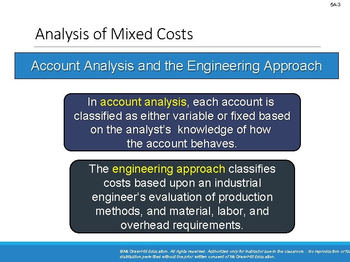
5 A-3 Analysis of Mixed Costs Account Analysis and the Engineering Approach In account analysis, each account is classified as either variable or fixed based on the analyst’s knowledge of how the account behaves. The engineering approach classifies costs based upon an industrial engineer’s evaluation of production methods, and material, labor, and overhead requirements. ©Mc. Graw-Hill Education. All rights reserved. Authorized only for instructor use in the classroom. No reproduction or fur distribution permitted without the prior written consent of Mc. Graw-Hill Education.

5 A-4 Learning Objective 10 Analyze a mixed cost using a scattergraph plot and the high-low method. ©Mc. Graw-Hill Education. All rights reserved. Authorized only for instructor use in the classroom. No reproduction or fur distribution permitted without the prior written consent of Mc. Graw-Hill Education.

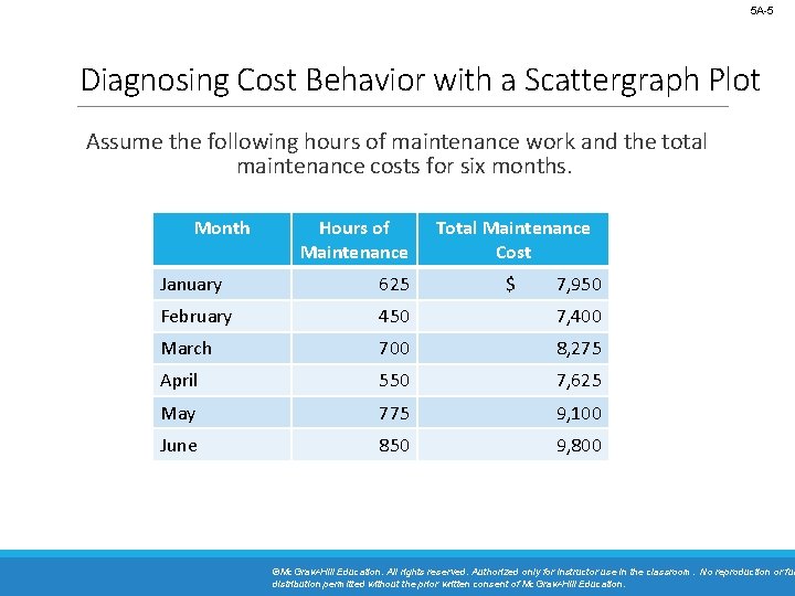
5 A-5 Diagnosing Cost Behavior with a Scattergraph Plot Assume the following hours of maintenance work and the total maintenance costs for six months. Month Hours of Maintenance Total Maintenance Cost January 625 $ 7, 950 February 450 7, 400 March 700 8, 275 April 550 7, 625 May 775 9, 100 June 850 9, 800 ©Mc. Graw-Hill Education. All rights reserved. Authorized only for instructor use in the classroom. No reproduction or fur distribution permitted without the prior written consent of Mc. Graw-Hill Education.

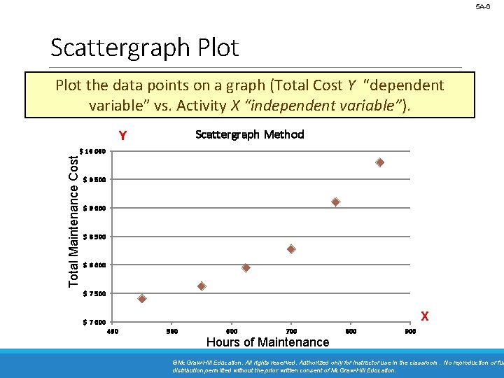
5 A-6 Scattergraph Plot the data points on a graph (Total Cost Y “dependent variable” vs. Activity X “independent variable”). Scattergraph Method Y Total Maintenance Cost $ 10 000 $ 9 500 $ 9 000 $ 8 500 $ 8 000 $ 7 500 $ 7 000 X 400 500 600 700 Hours of Maintenance 800 900 ©Mc. Graw-Hill Education. All rights reserved. Authorized only for instructor use in the classroom. No reproduction or fur distribution permitted without the prior written consent of Mc. Graw-Hill Education.

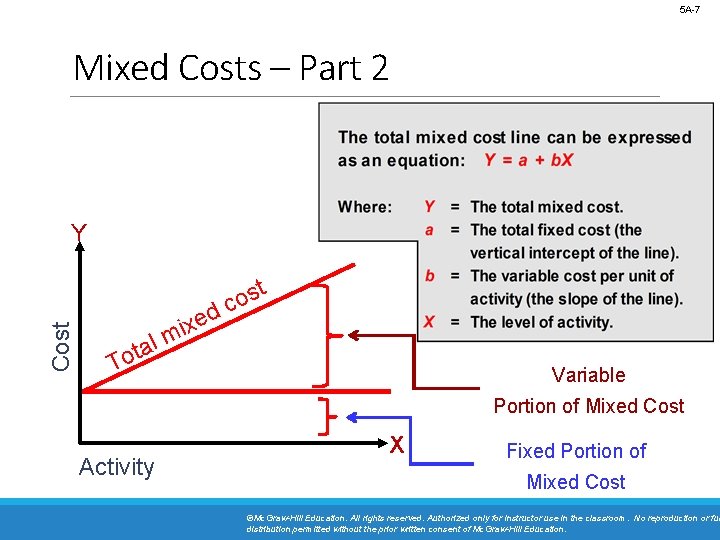
5 A-7 Mixed Costs – Part 2 Cost Y l a t o ed x i m t s o c T Variable Portion of Mixed Cost Activity X Fixed Portion of Mixed Cost ©Mc. Graw-Hill Education. All rights reserved. Authorized only for instructor use in the classroom. No reproduction or fur distribution permitted without the prior written consent of Mc. Graw-Hill Education.

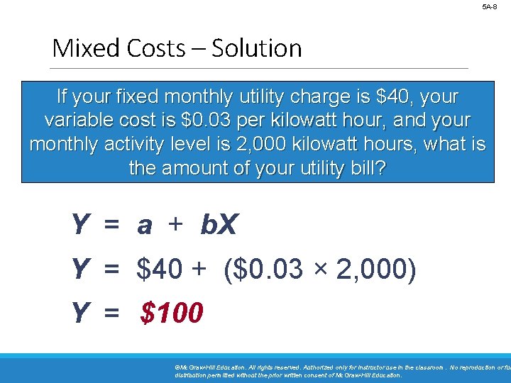
5 A-8 Mixed Costs – Solution If your fixed monthly utility charge is $40, your variable cost is $0. 03 per kilowatt hour, and your monthly activity level is 2, 000 kilowatt hours, what is the amount of your utility bill? Y = a + b. X Y = $40 + ($0. 03 × 2, 000) Y = $100 ©Mc. Graw-Hill Education. All rights reserved. Authorized only for instructor use in the classroom. No reproduction or fur distribution permitted without the prior written consent of Mc. Graw-Hill Education.

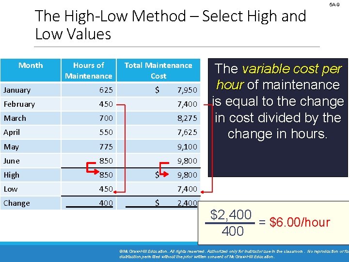
The High-Low Method – Select High and Low Values Month Hours of Maintenance Total Maintenance Cost January 625 $ February 450 7, 400 March 700 8, 275 April 550 7, 625 May 775 9, 100 June 850 9, 800 High 850 Low 450 Change 400 $ 7, 950 5 A-9 The variable cost per hour of maintenance is equal to the change in cost divided by the change in hours. 9, 800 7, 400 $ 2, 400 $2, 400 = $6. 00/hour 400 ©Mc. Graw-Hill Education. All rights reserved. Authorized only for instructor use in the classroom. No reproduction or fur distribution permitted without the prior written consent of Mc. Graw-Hill Education.

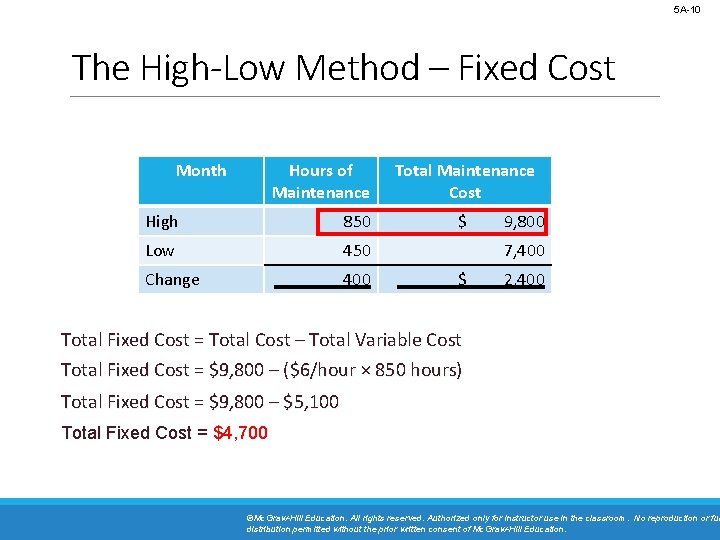
5 A-10 The High-Low Method – Fixed Cost Month Hours of Maintenance High 850 Low 450 Change 400 Total Maintenance Cost $ 9, 800 7, 400 $ 2, 400 Total Fixed Cost = Total Cost – Total Variable Cost Total Fixed Cost = $9, 800 – ($6/hour × 850 hours) Total Fixed Cost = $9, 800 – $5, 100 Total Fixed Cost = $4, 700 ©Mc. Graw-Hill Education. All rights reserved. Authorized only for instructor use in the classroom. No reproduction or fur distribution permitted without the prior written consent of Mc. Graw-Hill Education.

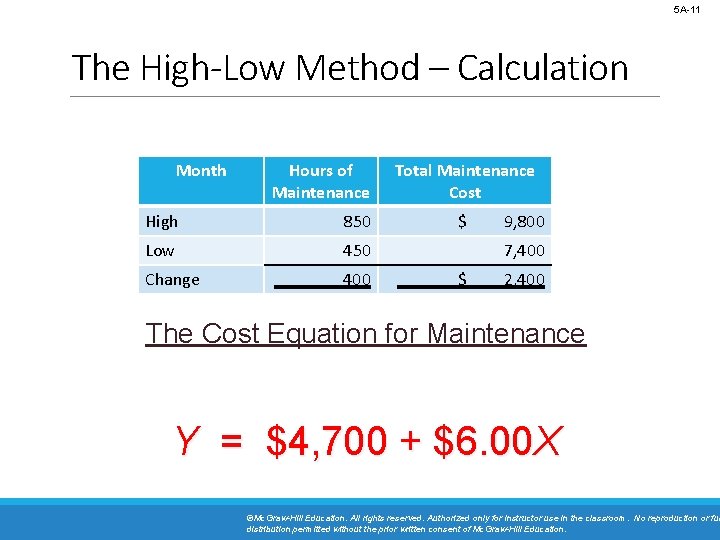
5 A-11 The High-Low Method – Calculation Month Hours of Maintenance High 850 Low 450 Change 400 Total Maintenance Cost $ 9, 800 7, 400 $ 2, 400 The Cost Equation for Maintenance Y = $4, 700 + $6. 00 X ©Mc. Graw-Hill Education. All rights reserved. Authorized only for instructor use in the classroom. No reproduction or fur distribution permitted without the prior written consent of Mc. Graw-Hill Education.

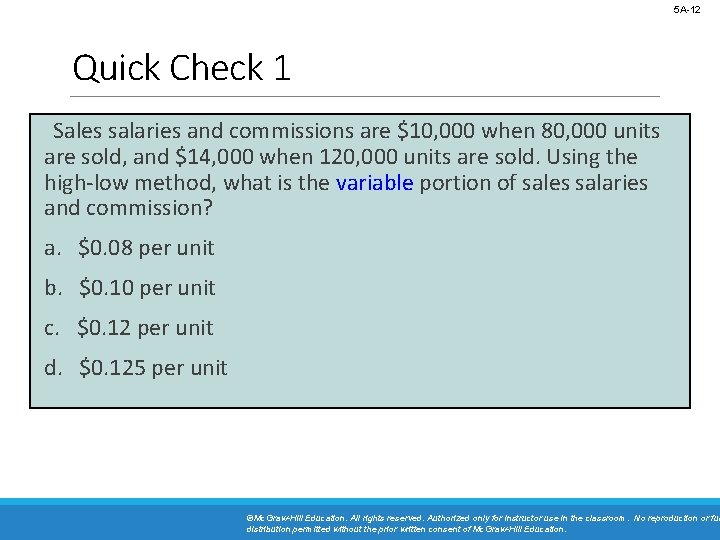
5 A-12 Quick Check 1 Sales salaries and commissions are $10, 000 when 80, 000 units are sold, and $14, 000 when 120, 000 units are sold. Using the high-low method, what is the variable portion of sales salaries and commission? a. $0. 08 per unit b. $0. 10 per unit c. $0. 12 per unit d. $0. 125 per unit ©Mc. Graw-Hill Education. All rights reserved. Authorized only for instructor use in the classroom. No reproduction or fur distribution permitted without the prior written consent of Mc. Graw-Hill Education.

5 A-13 Quick Check 1 a Sales salaries and commissions are $10, 000 when 80, 000 units are sold, and $14, 000 when 120, 000 units are sold. Using the high-low method, what is the variable portion of sales salaries and commission? a. $0. 08 per unit b. $0. 10 per unit $4, 000 ÷ 40, 000 units = $0. 10 per unit c. $0. 12 per unit d. $0. 125 per unit ©Mc. Graw-Hill Education. All rights reserved. Authorized only for instructor use in the classroom. No reproduction or fur distribution permitted without the prior written consent of Mc. Graw-Hill Education.

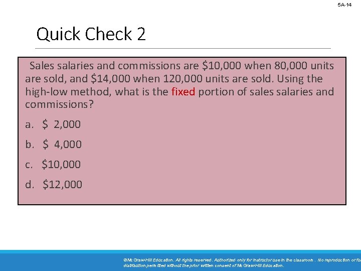
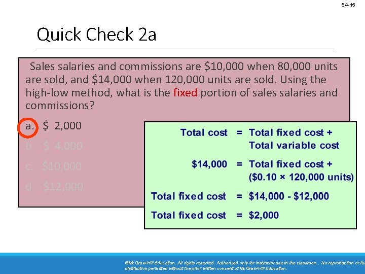
5 A-14 Quick Check 2 Sales salaries and commissions are $10, 000 when 80, 000 units are sold, and $14, 000 when 120, 000 units are sold. Using the high-low method, what is the fixed portion of sales salaries and commissions? a. $ 2, 000 b. $ 4, 000 c. $10, 000 d. $12, 000 ©Mc. Graw-Hill Education. All rights reserved. Authorized only for instructor use in the classroom. No reproduction or fur distribution permitted without the prior written consent of Mc. Graw-Hill Education.

5 A-15 Quick Check 2 a Sales salaries and commissions are $10, 000 when 80, 000 units are sold, and $14, 000 when 120, 000 units are sold. Using the high-low method, what is the fixed portion of sales salaries and commissions? a. $ 2, 000 b. $ 4, 000 c. $10, 000 d. $12, 000 ©Mc. Graw-Hill Education. All rights reserved. Authorized only for instructor use in the classroom. No reproduction or fur distribution permitted without the prior written consent of Mc. Graw-Hill Education.

5 A-16 Learning Objective 11 Analyze a mixed cost using a scattergraph plot and the least-squares regression method ©Mc. Graw-Hill Education. All rights reserved. Authorized only for instructor use in the classroom. No reproduction or fur distribution permitted without the prior written consent of Mc. Graw-Hill Education.

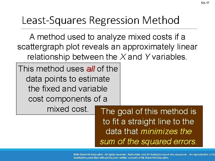
5 A-17 Least-Squares Regression Method A method used to analyze mixed costs if a scattergraph plot reveals an approximately linear relationship between the X and Y variables. This method uses all of the data points to estimate the fixed and variable cost components of a mixed cost. The goal of this method is to fit a straight line to the data that minimizes the sum of the squared errors. ©Mc. Graw-Hill Education. All rights reserved. Authorized only for instructor use in the classroom. No reproduction or fur distribution permitted without the prior written consent of Mc. Graw-Hill Education.

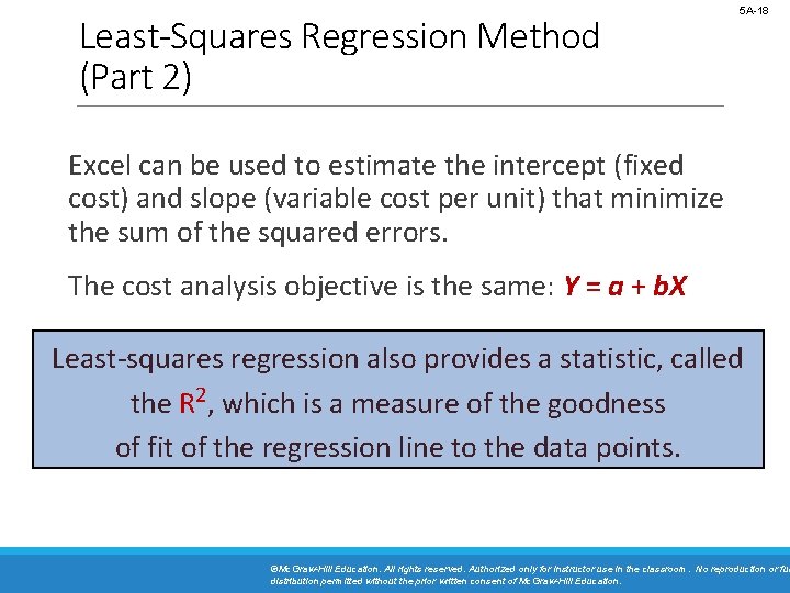
Least-Squares Regression Method (Part 2) 5 A-18 Excel can be used to estimate the intercept (fixed cost) and slope (variable cost per unit) that minimize the sum of the squared errors. The cost analysis objective is the same: Y = a + b. X Least-squares regression also provides a statistic, called the R 2, which is a measure of the goodness of fit of the regression line to the data points. ©Mc. Graw-Hill Education. All rights reserved. Authorized only for instructor use in the classroom. No reproduction or fur distribution permitted without the prior written consent of Mc. Graw-Hill Education.

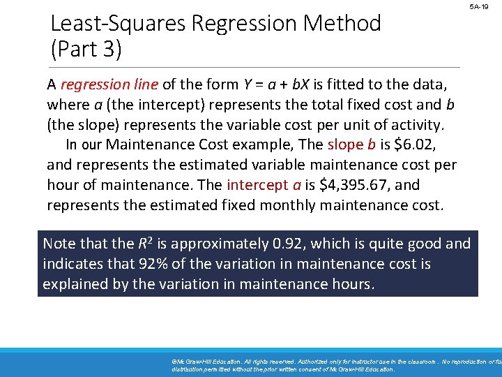
Least-Squares Regression Method (Part 3) 5 A-19 A regression line of the form Y = a + b. X is fitted to the data, where a (the intercept) represents the total fixed cost and b (the slope) represents the variable cost per unit of activity. In our Maintenance Cost example, The slope b is $6. 02, and represents the estimated variable maintenance cost per hour of maintenance. The intercept a is $4, 395. 67, and represents the estimated fixed monthly maintenance cost. Note that the R 2 is approximately 0. 92, which is quite good and indicates that 92% of the variation in maintenance cost is explained by the variation in maintenance hours. ©Mc. Graw-Hill Education. All rights reserved. Authorized only for instructor use in the classroom. No reproduction or fur distribution permitted without the prior written consent of Mc. Graw-Hill Education.

5 A-20 Comparing Results From the Two Methods The two methods just discussed provide different estimates of the fixed and variable cost components of a mixed cost. This is to be expected because each method uses differing amounts of the data points to provide estimates. Least-squares regression provides the most accurate estimate because it uses all the data points. ©Mc. Graw-Hill Education. All rights reserved. Authorized only for instructor use in the classroom. No reproduction or fur distribution permitted without the prior written consent of Mc. Graw-Hill Education.

5 A-21 End of Appendix 5 A ©Mc. Graw-Hill Education. All rights reserved. Authorized only for instructor use in the classroom. No reproduction or fur distribution permitted without the prior written consent of Mc. Graw-Hill Education.