Analyzing Measurement Data ENGR 1181 Class 8 Analyzing

Analyzing Measurement Data ENGR 1181 Class 8

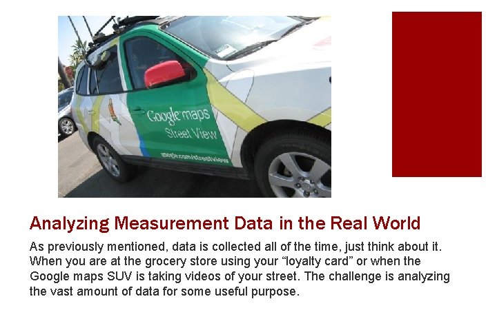
Analyzing Measurement Data in the Real World As previously mentioned, data is collected all of the time, just think about it. When you are at the grocery store using your “loyalty card” or when the Google maps SUV is taking videos of your street. The challenge is analyzing the vast amount of data for some useful purpose.

Today's Learning Objectives § After today’s class, students will be able to: • Define the terms mean, median, mode, central tendency, and standard deviation. • Analyze data using mean, median, and mode. • Determine the cause of variation in a given data set. • Identify whether variation in a given data set is systematic or random. • Identify outliers in a given data set. • Create a histogram for a given data set by determining an appropriate bin size and range.

Important Takeaways from Preparation Reading § Histograms • They depict data distribution • Must know # data points • Determine # of bins and bin size § Measures of Central Tendency § Measures of Variation

Analyzing Measurement Data When collecting data, there will always be variation. We can use statistical tools to help us determine: § Is the variation systematic or random? § What is the cause of the variation? § Is the variation in an acceptable range? § What is an acceptable range of variation for this data?

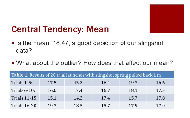
Example: Slingshot Experiment! An engineer is performing a data collection experiment using a slingshot and a softball. She predicted that if the slingshot is pulled back by 1 meter before launching the ball, the softball would land 17 meters downrange. Data is collected from 20 trials. Let’s analyze the data and see how the experiment went…

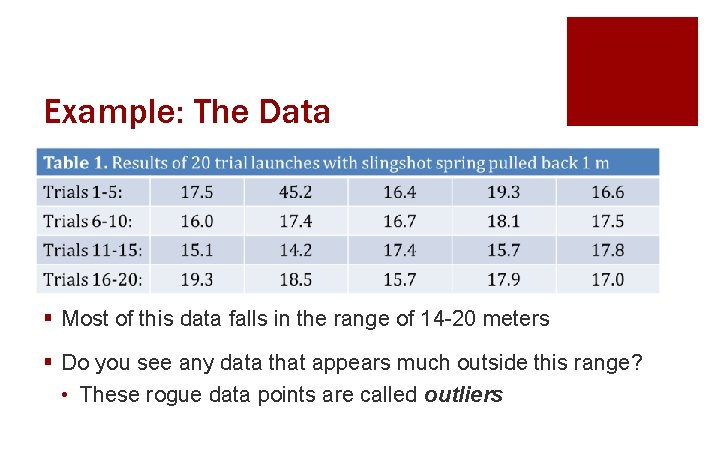
Example: The Data § Most of this data falls in the range of 14 -20 meters § Do you see any data that appears much outside this range? • These rogue data points are called outliers

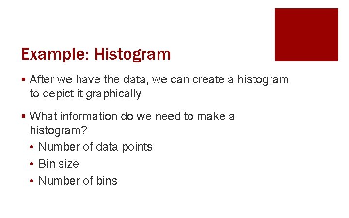
Example: Histogram § After we have the data, we can create a histogram to depict it graphically § What information do we need to make a histogram? • Number of data points • Bin size • Number of bins

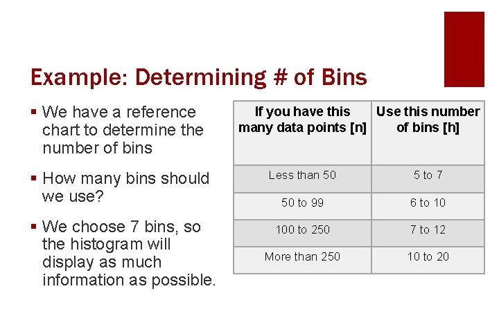
Example: Determining # of Bins § We have a reference chart to determine the number of bins § How many bins should we use? § We choose 7 bins, so the histogram will display as much information as possible. If you have this Use this number many data points [n] of bins [h] Less than 50 5 to 7 50 to 99 6 to 10 100 to 250 7 to 12 More than 250 10 to 20

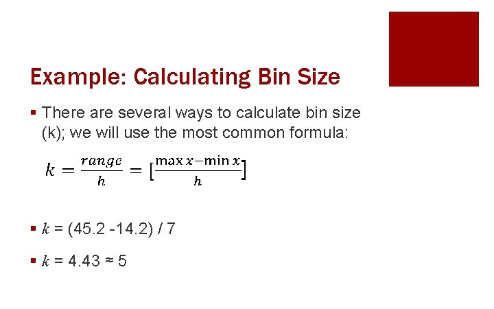
Example: Calculating Bin Size § There are several ways to calculate bin size (k); we will use the most common formula: § k = (45. 2 -14. 2) / 7 § k = 4. 43 ≈ 5

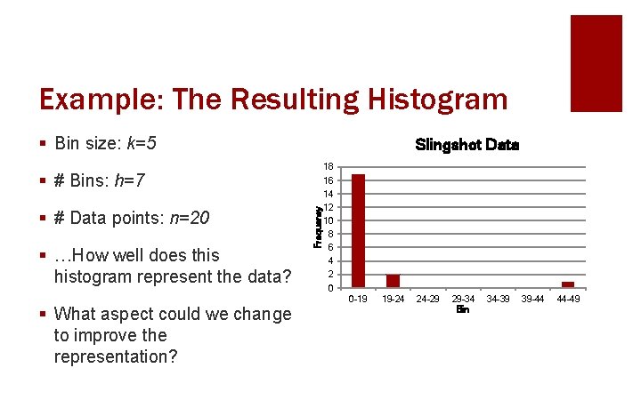
Example: The Resulting Histogram § Bin size: k=5 Slingshot Data 18 § # Bins: h=7 § …How well does this histogram represent the data? 14 Frequency § # Data points: n=20 16 12 10 8 6 4 2 0 0 -19 § What aspect could we change to improve the representation? 19 -24 24 -29 29 -34 Bin 34 -39 39 -44 44 -49

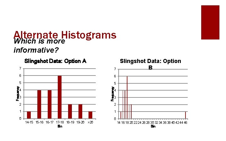
Alternate Histograms Which is more informative? 7 7 6 6 5 5 Frequency Slingshot Data: Option A 4 3 2 2 1 1 0 Slingshot Data: Option B 0 14 -15 15 -16 16 -17 17 -18 18 -19 19 -20 Bin >20 14 16 18 20 22 24 26 28 30 32 34 36 38 40 42 44 46 Bin

Histograms: A Summary § It is important that histograms accurately and thoroughly depict the data set § Sometimes the suggested number of bins or bin size will not fit the data set - use your judgment to make manual adjustments § Consider several options to ensure your histogram is as descriptive as possible

Outliers: Deal With It. § Outliers will happen even in good data sets. Good engineers know how to deal with them! § Engineers must determine whether an outlier is a valid data point, or if it is an error and thus invalid. § Invalid data points can be the result of measurement errors or of incorrectly recording the data.

Characterizing The Data § Statistics allows us to characterize the data numerically as well as graphically. § We characterize data numerically in two ways: • Central Tendency • Variation

Central Tendency § This is a single value that best represents the data. This value could be determined by: • Mean • Median • Mode § For many engineering applications, the mean and median are most relevant.

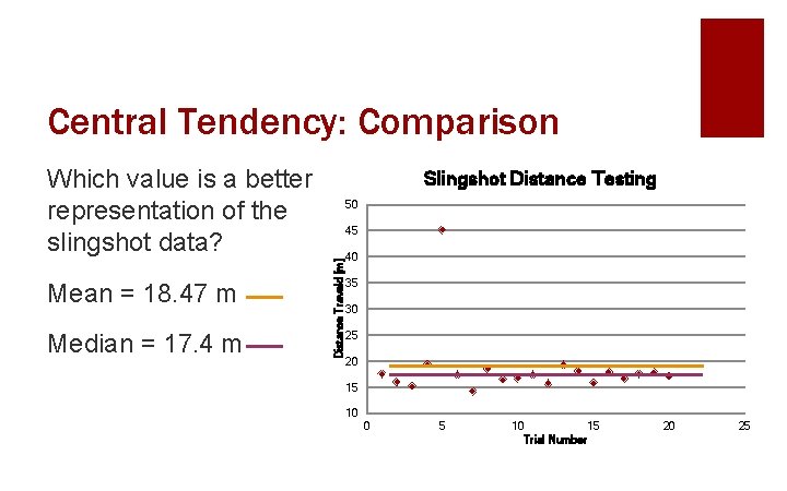
Central Tendency: Mean § Is the mean, 18. 47, a good depiction of our slingshot data? § What about the outlier? How does that affect our mean?

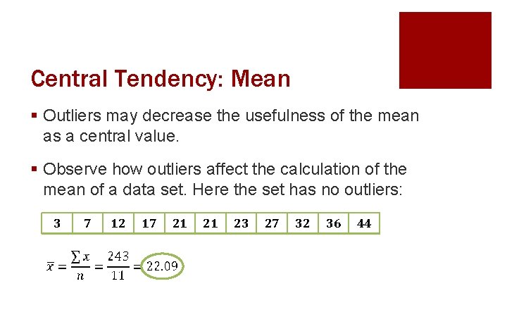
Central Tendency: Mean § Outliers may decrease the usefulness of the mean as a central value. § Observe how outliers affect the calculation of the mean of a data set. Here the set has no outliers: 3 7 12 17 21 21 23 27 32 36 44

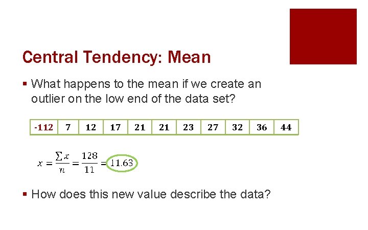
Central Tendency: Mean § What happens to the mean if we create an outlier on the low end of the data set? -112 7 12 17 21 21 23 27 32 36 § How does this new value describe the data? 44

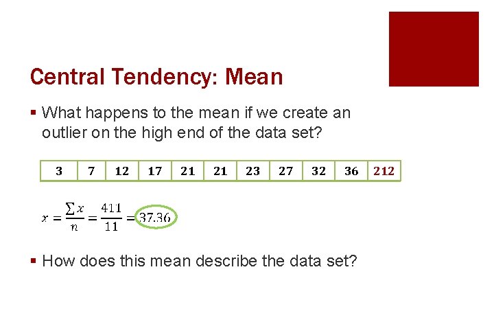
Central Tendency: Mean § What happens to the mean if we create an outlier on the high end of the data set? 3 7 12 17 21 21 23 27 32 36 § How does this mean describe the data set? 212

What Does It All Mean? ! § When outliers are present, sometimes the mean is not the best characterization of the data. § What is another value we could use? • The Median!

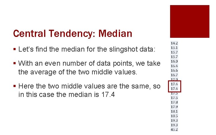
Central Tendency: Median § Let’s find the median for the slingshot data: § With an even number of data points, we take the average of the two middle values. § Here the two middle values are the same, so in this case the median is 17. 4

Central Tendency: Comparison Which value is a better representation of the slingshot data? Median = 17. 4 m 50 45 Distance Traveld [m] Mean = 18. 47 m Slingshot Distance Testing 40 35 30 25 20 15 10 0 5 10 15 Trial Number 20 25

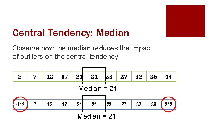
Central Tendency: Median Observe how the median reduces the impact of outliers on the central tendency: Median = 21

Characterizing the Data § We can select a value of central tendency to represent the data, but is just one number enough? § No! It is also important to know how much variation is present in the data. § Variation describes how the data is distributed around the central tendency value.

Representing Variation § As with central tendency, there are multiple ways to represent variation in a set of data: • ± (“Plus/Minus”) gives the range of values • Standard Deviation provides a more sophisticated look at how the data is distributed around the central value.

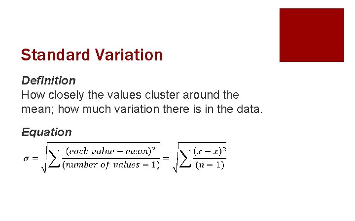
Standard Variation Definition How closely the values cluster around the mean; how much variation there is in the data. Equation

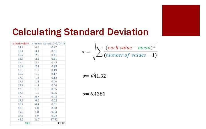
Calculating Standard Deviation

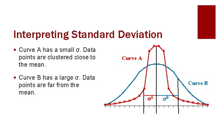
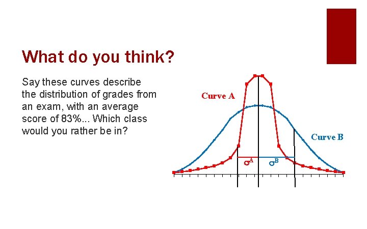
Interpreting Standard Deviation § Curve A has a small σ. Data points are clustered close to the mean. § Curve B has a large σ. Data points are far from the mean. Curve A Curve B A B

What do you think? Say these curves describe the distribution of grades from an exam, with an average score of 83%. . . Which class would you rather be in? Curve A Curve B A B

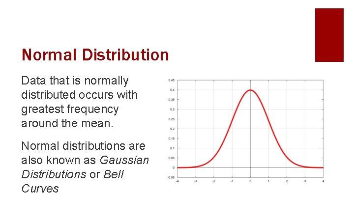
Normal Distribution Data that is normally distributed occurs with greatest frequency around the mean. Normal distributions are also known as Gaussian Distributions or Bell Curves

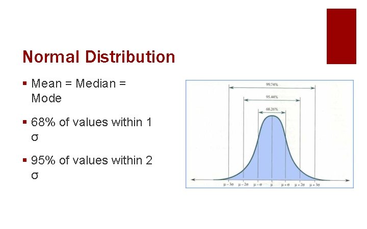
Normal Distribution § Mean = Median = Mode § 68% of values within 1 σ § 95% of values within 2 σ

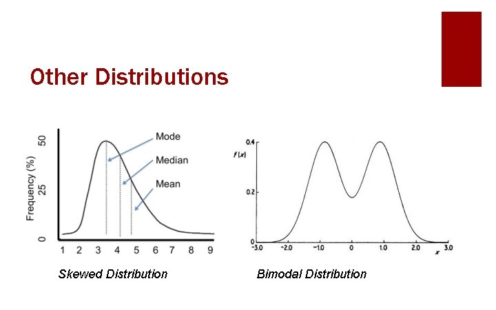
Other Distributions Skewed Distribution Bimodal Distribution

Important Takeaways § We have learned about some basic statistical tools that engineers use to analyze data. § Histograms are used to graphically represent data, but must be created thoughtfully. § Engineers use both central tendency and variation to numerically describe data.

Preview of Next Class § Technical Communication 2 • Expand on written technical communication, with a focus on writing lab memos and lab reports. • Discuss good and poor quality presentation material and verbal delivery of technical information.