ANALYZING DATA RELATIONSHIPS Objective of UI Profiling Systems

ANALYZING DATA RELATIONSHIPS

Objective of UI Profiling Systems To aid in the efficient identification of permanently laid off workers who are: Unlikely to return to previous industry or occupation Likely to exhaust regular UI benefits Need reemployment assistance to make a successful transition to new employment.

Profiling A systematic procedure used to ID UI claimants who, because of certain characteristics, are thought to be permanently separated from their prior job and likely to exhaust regular UI benefits.

Characteristic Screen A profiling methodology designed to use available data elements as the basis for including or excluding individual claimants from the target group based upon their particular profile.

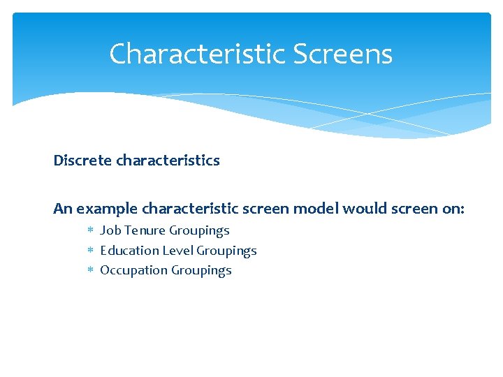
Characteristic Screens Discrete characteristics An example characteristic screen model would screen on: Job Tenure Groupings Education Level Groupings Occupation Groupings

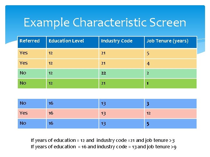
Example Characteristic Screen Referred Education Level Industry Code Job Tenure (years) Yes 12 21 5 Yes 12 21 4 No 12 22 2 No 12 21 1 No 16 13 3 Yes 16 13 12 No 16 13 5 If years of education = 12 and industry code =21 and job tenure >3 If years of education = 16 and industry code = 13 and job tenure >9

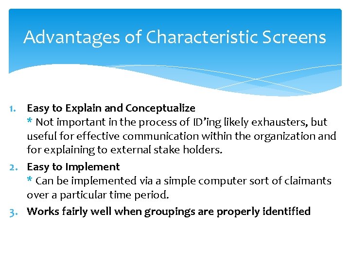
Advantages of Characteristic Screens 1. Easy to Explain and Conceptualize * Not important in the process of ID’ing likely exhausters, but useful for effective communication within the organization and for explaining to external stake holders. 2. Easy to Implement * Can be implemented via a simple computer sort of claimants over a particular time period. 3. Works fairly well when groupings are properly identified

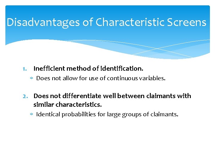
Disadvantages of Characteristic Screens 1. Inefficient method of identification. Does not allow for use of continuous variables. 2. Does not differentiate well between claimants with similar characteristics. Identical probabilities for large groups of claimants.

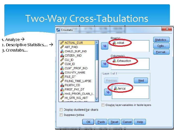
Two-Way Cross-Tabulations 1. Analyze 2. Descriptive Statistics… 3. Crosstabs…

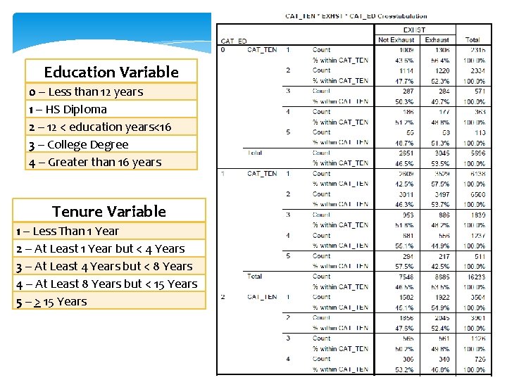
Education Variable 0 – Less than 12 years 1 – HS Diploma 2 – 12 < education years<16 3 – College Degree 4 – Greater than 16 years Tenure Variable 1 – Less Than 1 Year 2 – At Least 1 Year but < 4 Years 3 – At Least 4 Years but < 8 Years 4 – At Least 8 Years but < 15 Years 5 – > 15 Years

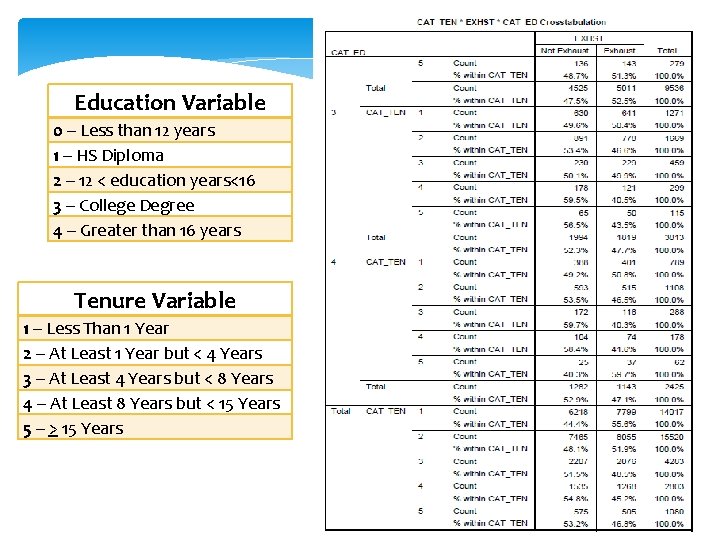
Education Variable 0 – Less than 12 years 1 – HS Diploma 2 – 12 < education years<16 3 – College Degree 4 – Greater than 16 years Tenure Variable 1 – Less Than 1 Year 2 – At Least 1 Year but < 4 Years 3 – At Least 4 Years but < 8 Years 4 – At Least 8 Years but < 15 Years 5 – > 15 Years

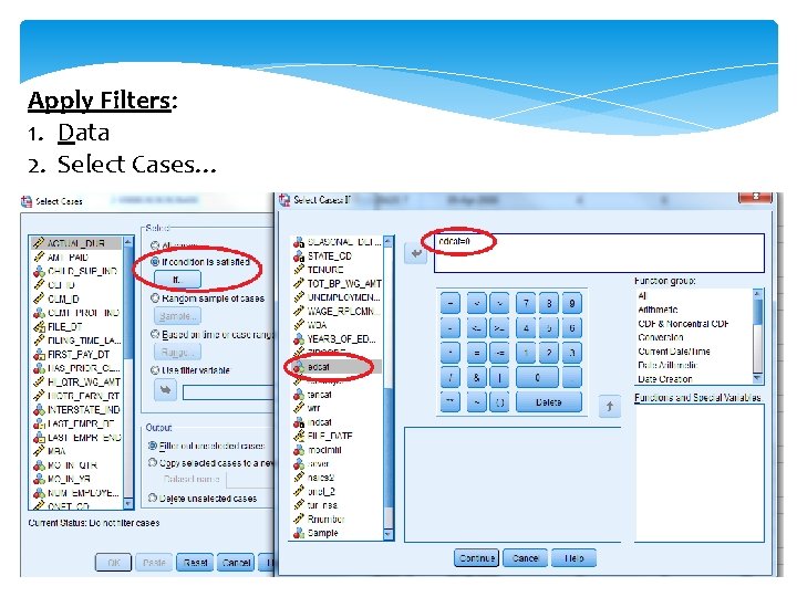
Apply Filters: 1. Data 2. Select Cases…

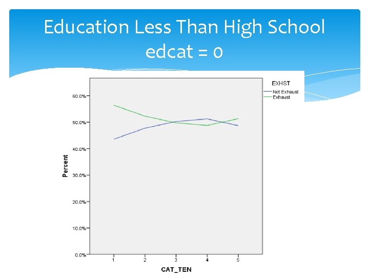
Education Less Than High School edcat = 0

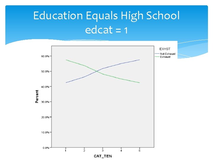
Education Equals High School edcat = 1

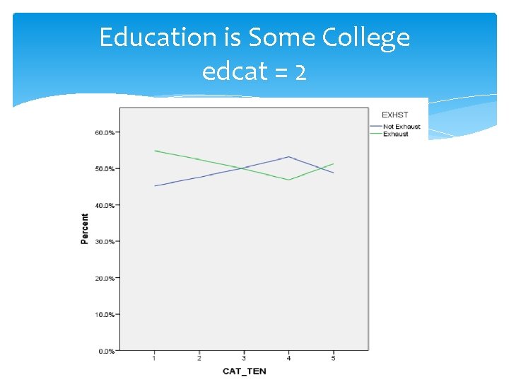
Education is Some College edcat = 2

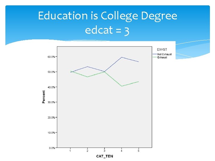
Education is College Degree edcat = 3

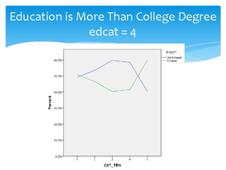
Education is More Than College Degree edcat = 4

Analysis of Graphs Highest Probability of Exhaustion: 0. 597 (59. 70%) for Education More Than College (edcat = 4) and Job Tenure > 15 years (tencat = 5) Lowest Probability of Exhaustion: 0. 403 (40. 3%) for Education More Than College (edcat = 4) and Job Tenure at least 4 years but < 8 years (tencat = 3)

Chi-Square Automatic Interaction Detection CHAID is… • a form of analysis that determines how variables best combine to explain the outcome in a given dependent variable. • a perfect tool to discover the relationship between variables. • a tool that can visualize the relationship between the target (dependent) variable and the related factors with a tree image.

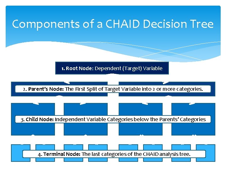
Components of a CHAID Decision Tree 1. Root Node: Dependent (Target) Variable 2. Parent’s Node: The First Split of Target Variable into 2 or more categories. 3. Child Node: Independent Variable Categories below the Parents’ Categories 4. Terminal Node: The last categories of the CHAID analysis tree.

Step 1: Preparing Variables • CHAID only accepts nominal or ordinal categorical predictors. When predictors are continuous, they are transformed into ordinal predictors. • Creates categorical predictors out of any continuous predictors by dividing the respective continuous distributions into a number of categories with an approximately equal number of observations. For categorical predictors, the categories (classes) are already defined.

Step 2: Merging • Cycle through the predictors to determine for each predictor the pair of (predictor) categories that is least significantly different with respect to the dependent variable. It does this by computing a Chi-square test (Pearson Chi-square). • For each predictor variable , merge non-significant categories. • Significant predictor categories (less than the respective alpha-to-merge value) will have a Bonferroni adjusted p-value computed for the set of categories of the respective predictor.

Step 3: Splitting The splitting step selects which predictor to be used to best split the node. Selection is accomplished by comparing the adjusted p-value associated with each predictor. • Choose the predictor variable with the smallest adjusted p-value, i. e. , the predictor variable that will yield the most significant split. • If this adjusted p-value is less than or equal to a user-specified alpha-level (alpha_split), split the node using this predictor. Else, do not split and the node is considered as a terminal node.

Step 4: Stopping The stopping step checks if the tree growing process should be stopped. The node will not be split if… • All cases in a node have identical values of the dependent variable • All cases in a node have identical values for each predictor • The current tree depth reaches the user specified maximum tree depth limit value • The size of a node is less than the user-specified minimum node size value • Resulting number of child nodes is 1 Continue this Steps 2 -3 until no further splits can be performed (given the alpha-tomerge and alpha-to-split values).

Classification & Regression Tree Analysis CART is the same as CHAID except only binary splits are allowed and uses pruning to adjust for tree size. CHAID is most useful for analysis, whereas CART is more suitable for prediction.

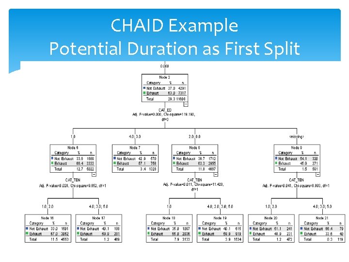
CHAID Example Potential Duration as First Split

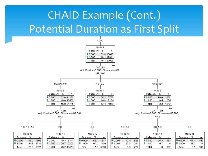
CHAID Example (Cont. ) Potential Duration as First Split

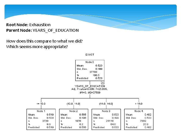
Root Node: Exhaustion Parent Node: YEARS_OF_EDUCATION How does this compare to what we did? Which seems more appropriate?

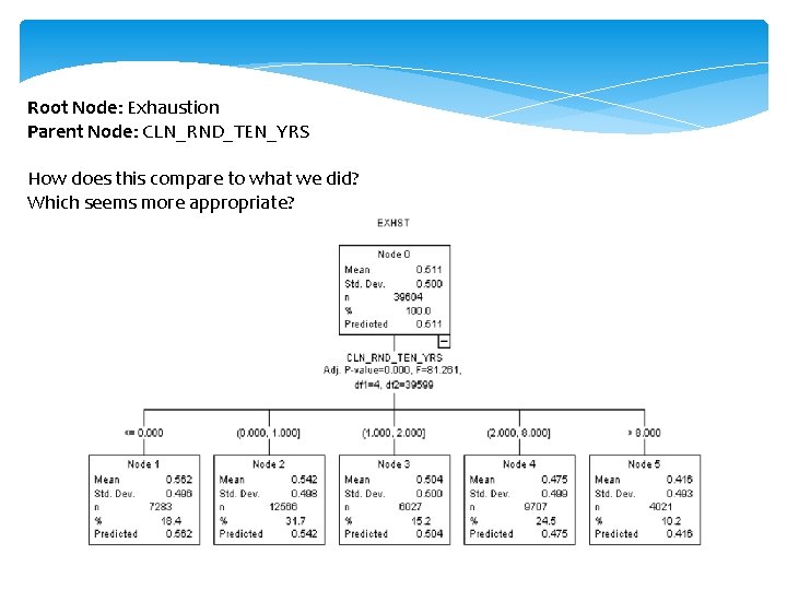
Root Node: Exhaustion Parent Node: CLN_RND_TEN_YRS How does this compare to what we did? Which seems more appropriate?

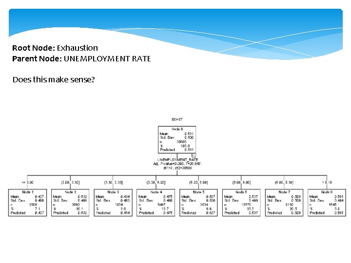
Root Node: Exhaustion Parent Node: UNEMPLOYMENT RATE Does this make sense?

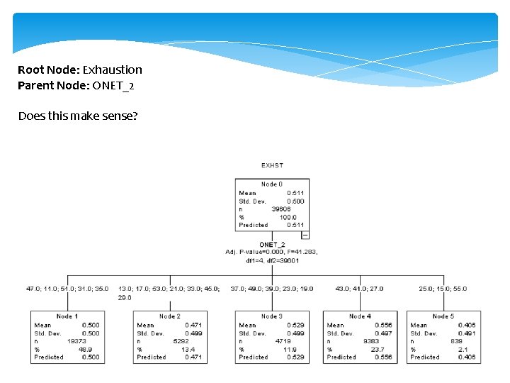
Root Node: Exhaustion Parent Node: ONET_2 Does this make sense?