Analyzing community data with joint species distribution models
Analyzing community data with joint species distribution models abundance, traits, phylogeny, co-occurrence and spatio-temporal structures Global Otso Ovaskainen University of Helsinki, Finland NTNU Trondheim, Norway
What structures the assembly and dynamics of communities? Leibold et al. (2004): The dynamics and distributions of communities are shaped by the interplay between i. environmental filtering ii. species interactions iii. spatial and stochastic processes Logue et al. (2011): Metacommunity theories are still poorly linked with data. There is a lack of statistical frameworks that would enable one to infer metacommunity processes from data typically available in community ecological studies.
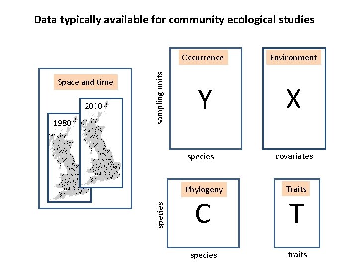
2000 1980 Occurrence Environment Y X species Space and time sampling units Data typically available for community ecological studies covariates Phylogeny Traits C T species traits
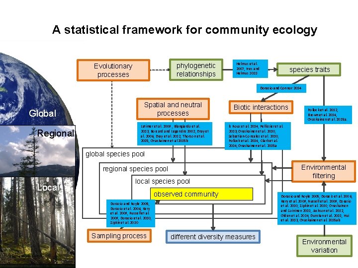
A statistical framework for community ecology phylogenetic relationships Evolutionary processes Helmus et al. 2007, Ives and Helmus 2011 species traits Dorazio and Connor 2014 Global Regional Spatial and neutral processes Latimer et al. 2009 , Blangiardo et al. 2013, Borcard and Legendre 2002, Dray et al. 2006, Dray et al. 2012, Thorson et al. 2015, Ovaskainen et al 2015 b Biotic interactions Pollock et al. 2012, Brown et al. 2014, Ovaskainen et al. 2015 a. le Roux et al. 2014, Pellissier et al. 2013, Ovaskainen et al. 2010, Sebastian-Gonzalez et al. 2010, Pollock et al. 2014, Clark et al. 2014, Ovaskainen et al. 2015 a global species pool regional species pool Local local species pool observed community Dorazio and Royle 2005, Dorazio et al. 2006, Kery et al. 2009, Russell et al. 2009, Dorazio et al. 2010, Zipkin et al. 2010 Sampling process different diversity measures Environmental filtering Dorazio and Royle 2005, Dorazio et al. 2006, Kery et al. 2009, Russell et al. 2009, Dorazio et al. 2010, Zipkin et al. 2010, Ovaskainen and Soininen 2011, Jackson et al. 2012, Olden et al. 2014, Dunstan et al. 2011, Hui et al. 2013, Ovaskainen et al. 2015 ab Environmental variation

2000 1980 Occurrence Environment Y X species Space and time sampling units SDM (species distribution model) covariates Phylogeny Traits C T species traits

SDM (species distribution model) Linear predictor for sampling unit j environmental covariates regression parameters Example link function: probit regression for presence-absence data Species occurrence: Latent occurrence score: Residual:

2000 1980 Occurrence Environment Y X species Space and time sampling units JSDM (joint species distribution model) covariates Phylogeny Traits C T species traits
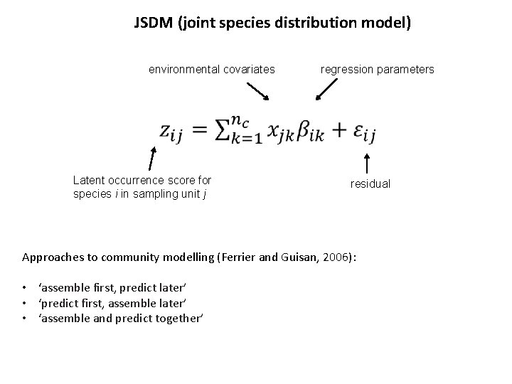
JSDM (joint species distribution model) environmental covariates regression parameters Latent occurrence score for species i in sampling unit j residual Approaches to community modelling (Ferrier and Guisan, 2006): • ‘assemble first, predict later’ • ‘predict first, assemble later’ • ‘assemble and predict together’
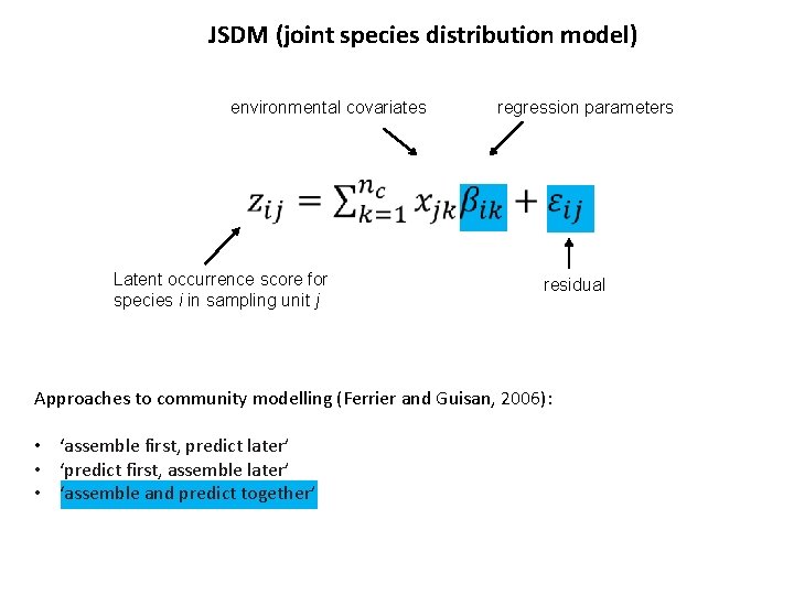
JSDM (joint species distribution model) environmental covariates regression parameters Latent occurrence score for species i in sampling unit j residual Approaches to community modelling (Ferrier and Guisan, 2006): • ‘assemble first, predict later’ • ‘predict first, assemble later’ • ‘assemble and predict together’
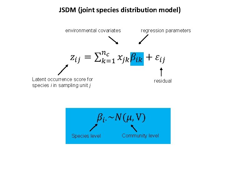
JSDM (joint species distribution model) environmental covariates regression parameters Latent occurrence score for species i in sampling unit j residual Species level Community level

Example: borrowing information from other species to parameterize models for rare species 500 diatom species surveyed for presenceabsence on 105 sampling units (streams) Number of species Training data: 35 sampling units Validation data: 70 sampling units training data full data independent models, prior 1 independent models, prior 2 community model, prior 1 community model, prior 2 Number of sites Ovaskainen and Soininen (Ecology, 2011) Oldén et al. (Plos one, 2014)
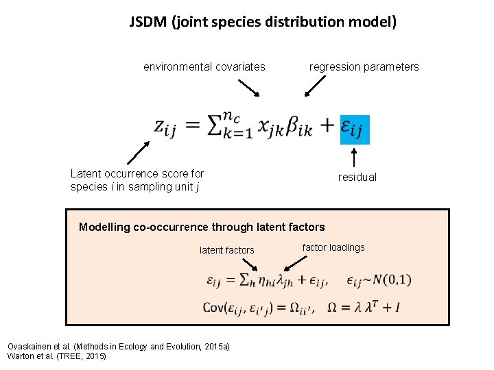
JSDM (joint species distribution model) environmental covariates regression parameters Latent occurrence score for species i in sampling unit j residual Modelling co-occurrence through latent factors Ovaskainen et al. (Methods in Ecology and Evolution, 2015 a) Warton et al. (TREE, 2015) factor loadings

Example: co-occurrence among wood-inhabiting fungi P(positive association)>0. 95 P(negative association)>0. 95 Ovaskainen et al. (Methods in Ecology and Evolution, 2015 a)
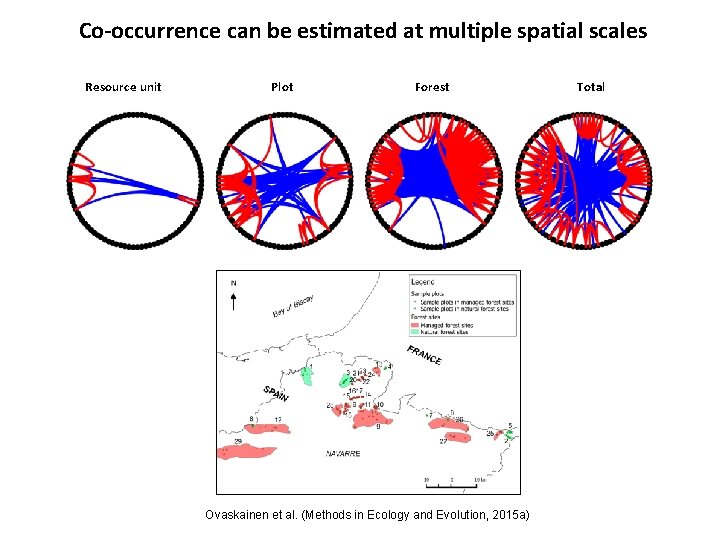
Co-occurrence can be estimated at multiple spatial scales Resource unit Plot Forest Ovaskainen et al. (Methods in Ecology and Evolution, 2015 a) Total
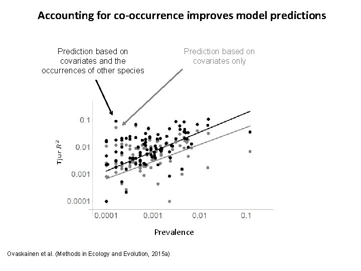
Accounting for co-occurrence improves model predictions Prediction based on covariates only Prediction based on covariates and the occurrences of other species Prevalence Ovaskainen et al. (Methods in Ecology and Evolution, 2015 a)
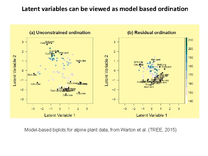
Latent variables can be viewed as model based ordination Model-based biplots for alpine plant data, from Warton et al. (TREE, 2015)
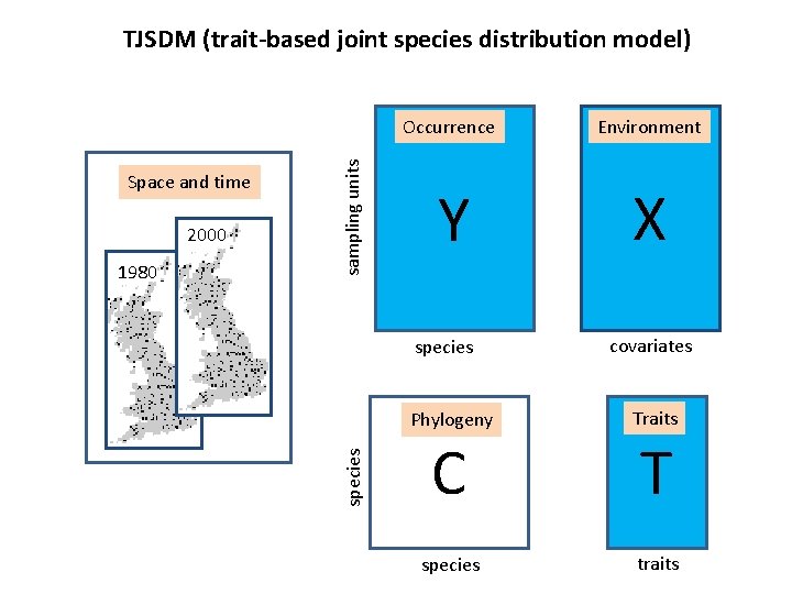
2000 1980 Occurrence Environment Y X species Space and time sampling units TJSDM (trait-based joint species distribution model) covariates Phylogeny Traits C T species traits
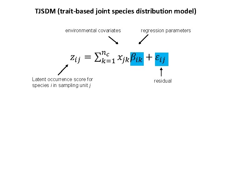
TJSDM (trait-based joint species distribution model) environmental covariates regression parameters Latent occurrence score for species i in sampling unit j residual
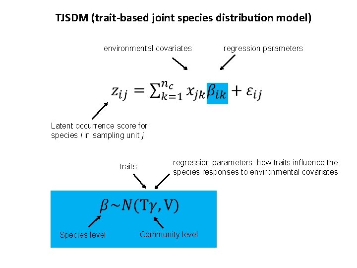
TJSDM (trait-based joint species distribution model) environmental covariates regression parameters Latent occurrence score for species i in sampling unit j traits regression parameters: how traits influence the species responses to environmental covariates Species level Community level
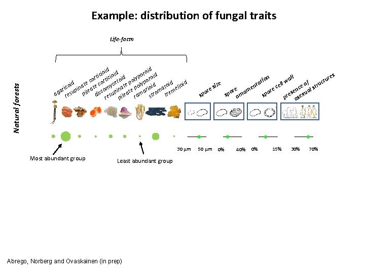
Example: distribution of fungal traits Natural forests Life-form d d roi id ioi oid c o i i t p d o cor ortic etoi poly ypor e d id id c c i t l e co pina ate omy inat e po rioid ato ello i r e a m m ag resu pil disc esup ileat rama stro tre r p 30 µm Most abundant group Least abundant group Abrego, Norberg and Ovaskainen (in prep) s ll wa ure t c f l e u o t siz cel en ce al str e e e n r m r r e s u spo orna spo pre asex on ati 50 µm 0% 40% 0% 15% 30% 70%
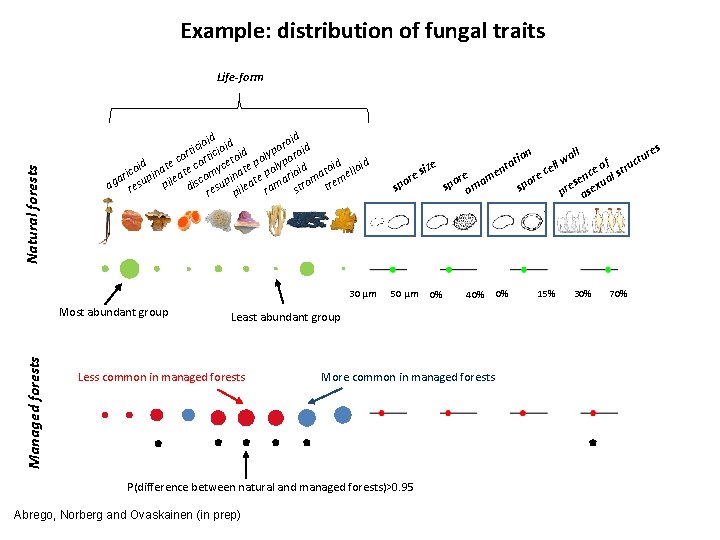
Example: distribution of fungal traits Natural forests Life-form d d roi id ioi oid c o i i t p d o cor ortic etoi poly ypor e d id id c c i t l e co pina ate omy inat e po rioid ato ello i r e a m m ag resu pil disc esup ileat rama stro tre r p 30 µm Managed forests Most abundant group ure t c f l e u o t siz cel en ce al str e e e n r m r r e s u spo orna spo pre asex 50 µm 0% 40% Least abundant group Less common in managed forests More common in managed forests P(difference between natural and managed forests)>0. 95 Abrego, Norberg and Ovaskainen (in prep) s ll wa on ati 0% 15% 30% 70%
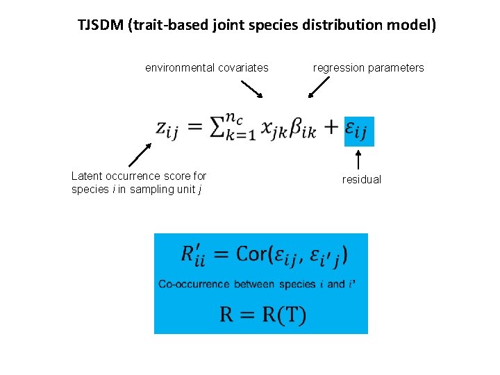
TJSDM (trait-based joint species distribution model) environmental covariates regression parameters Latent occurrence score for species i in sampling unit j residual
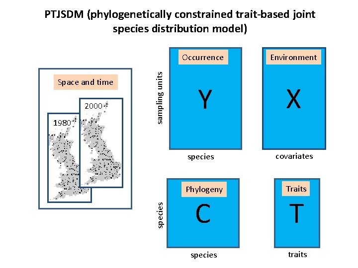
2000 1980 Occurrence Environment Y X species Space and time sampling units PTJSDM (phylogenetically constrained trait-based joint species distribution model) covariates Phylogeny Traits C T species traits
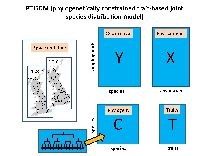
2000 1980 Occurrence Environment Y X species Space and time sampling units PTJSDM (phylogenetically constrained trait-based joint species distribution model) covariates Phylogeny Traits C T species traits
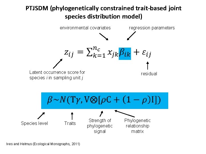
PTJSDM (phylogenetically constrained trait-based joint species distribution model) environmental covariates regression parameters Latent occurrence score for species i in sampling unit j residual Species level Traits Ives and Helmus (Ecological Monographs, 2011) Strength of phylogenetic signal Phylogenetic relationship matrix
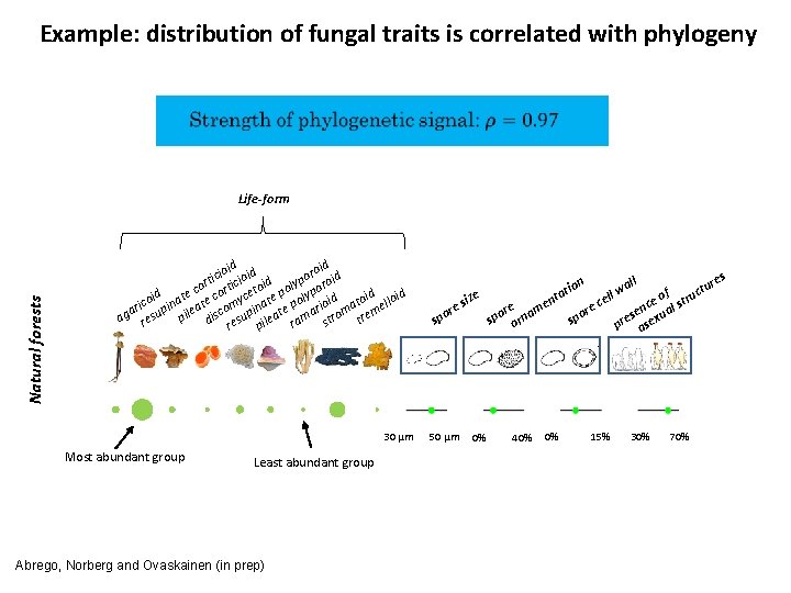
Example: distribution of fungal traits is correlated with phylogeny Natural forests Life-form d d roi id ioi oid c o i i t p d o cor ortic etoi poly ypor e d id id c c i t l e co pina ate omy inat e po rioid ato ello i r e a m m ag resu pil disc esup ileat rama stro tre r p 30 µm Most abundant group Least abundant group Abrego, Norberg and Ovaskainen (in prep) ize s ore sp 50 µm 0% n io tat en re m spo orna 40% 0% res ll a ll w tu of truc e e c s c re en xual o s p e s pr ase 15% 30% 70%
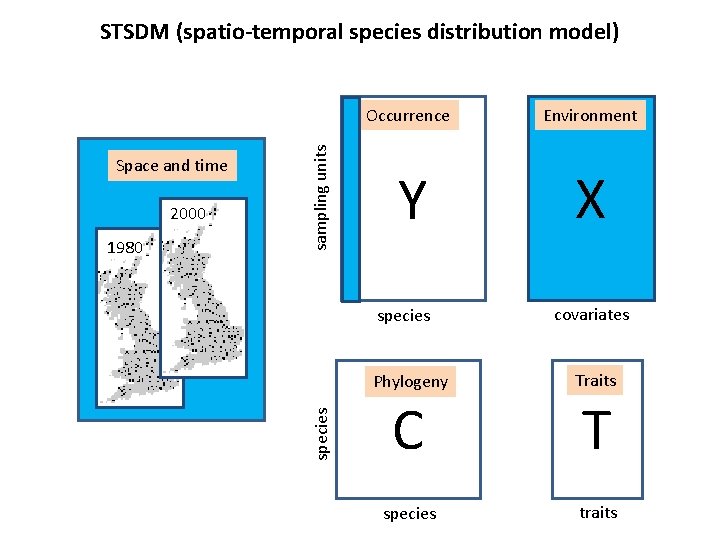
2000 1980 Occurrence Environment Y X species Space and time sampling units STSDM (spatio-temporal species distribution model) covariates Phylogeny Traits C T species traits
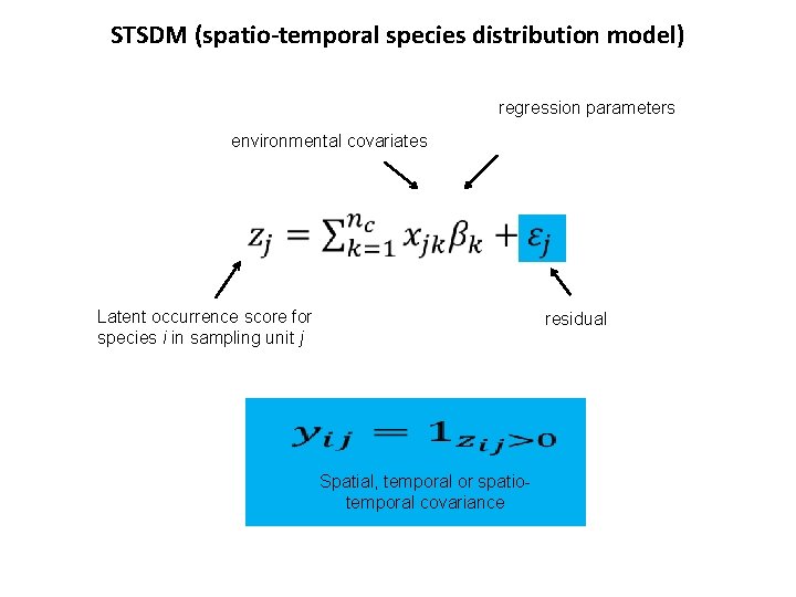
STSDM (spatio-temporal species distribution model) regression parameters environmental covariates Latent occurrence score for species i in sampling unit j residual Spatial, temporal or spatiotemporal covariance
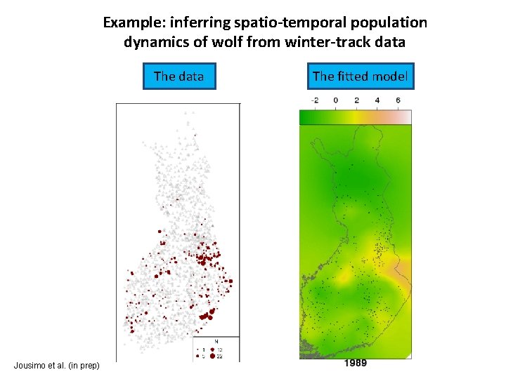
Example: inferring spatio-temporal population dynamics of wolf from winter-track data The data Jousimo et al. (in prep) The fitted model
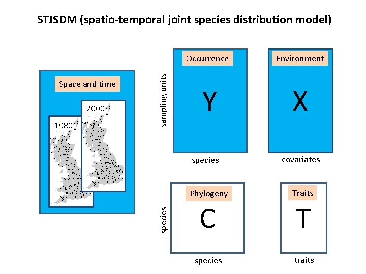
2000 1980 Occurrence Environment Y X species Space and time sampling units STJSDM (spatio-temporal joint species distribution model) covariates Phylogeny Traits C T species traits
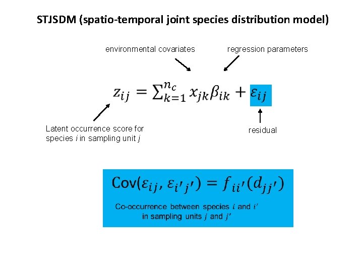
STJSDM (spatio-temporal joint species distribution model) environmental covariates regression parameters Latent occurrence score for species i in sampling unit j residual
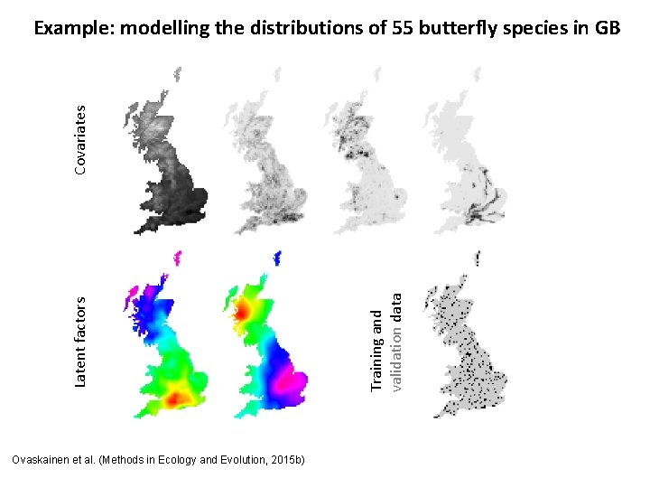
Ovaskainen et al. (Methods in Ecology and Evolution, 2015 b) Training and validation data Latent factors Covariates Example: modelling the distributions of 55 butterfly species in GB
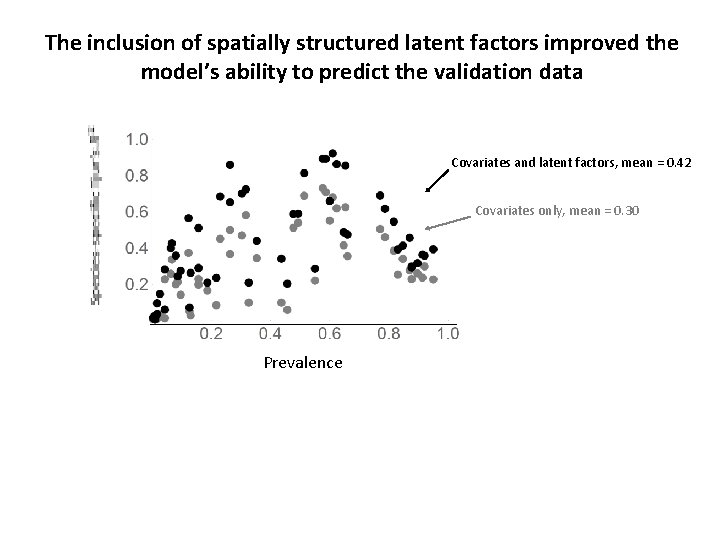
The inclusion of spatially structured latent factors improved the model’s ability to predict the validation data Covariates and latent factors, mean = 0. 42 Covariates only, mean = 0. 30 Prevalence
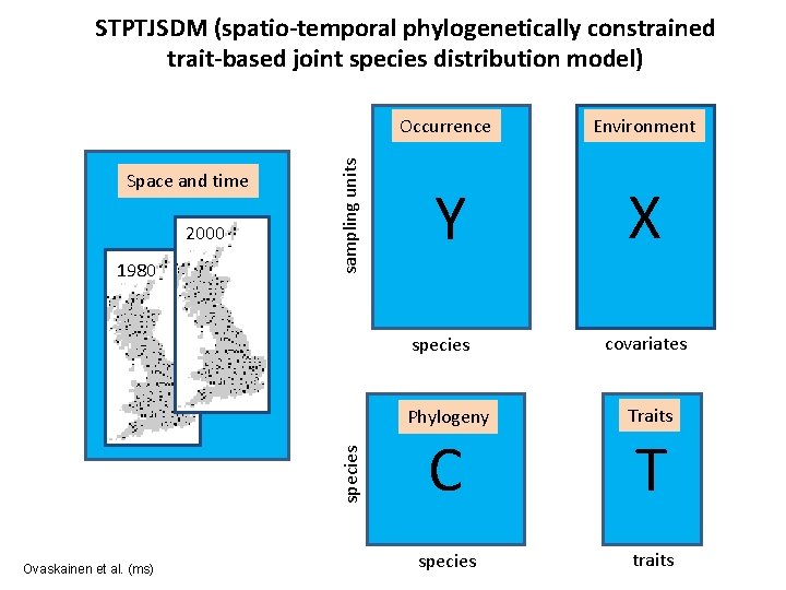
Space and time 2000 1980 sampling units STPTJSDM (spatio-temporal phylogenetically constrained trait-based joint species distribution model) Occurrence Environment Y X species Ovaskainen et al. (ms) covariates Phylogeny Traits C T species traits
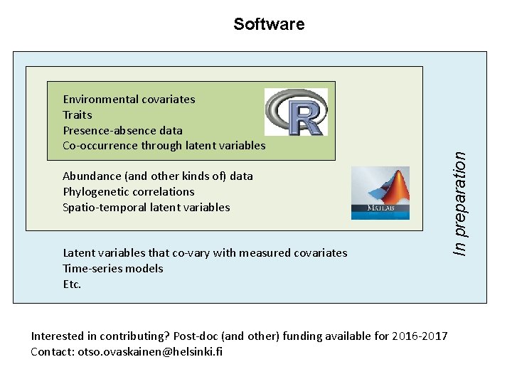
Environmental covariates Traits Presence-absence data Co-occurrence through latent variables Abundance (and other kinds of) data Phylogenetic correlations Spatio-temporal latent variables Latent variables that co-vary with measured covariates Time-series models Etc. Interested in contributing? Post-doc (and other) funding available for 2016 -2017 Contact: otso. ovaskainen@helsinki. fi In preparation Software
Conclusions • There is a lack of statistical frameworks that would enable one to infer metacommunity processes from data typically available in community ecological studies. • Joint species distribution modelling is one fast developing area which tries to fill this gap. Global • A lot of relevant structures can be built into generalized hierarchical linear mixed models: hierarchical layers, covariance structures, error structures and link functions. • The joint species distribution models presented here are of general nature and thus applicable to many kinds of study systems and study questions. • More refined information on specific systems may be obtained by other approaches (e. g. process-based state-space models).
- Slides: 36