Analytic techniques for nonlinear PDEs Group C Introduction

Analytic techniques for nonlinear PDEs Group C

Introduction Non linear partial differential equations are (as their name suggests) Partial differential equations with nonlinear terms. They describe many different physical systems, ranging from gravitation to fluid dynamics, and have been used in mathematics to solve problems (such as the Poincaré conjecture and the Calabi conjecture). They are difficult to study: there almost no general techniques that work for all such equations, and usually each individual equation has to be studied as a separate problem.

There are various techniques of non linear PDEs but each technique is limited to only a small class of non linear PDEs. A brief intro of the following techinques is given in this presentation. • • Conservation Law and Shock Inverse Scattering Transform Lax-Pair Formalism Bi-Hamiltonian Theory

Conversation Law And Shock

Introduction • Most field equations in engineering stem from balance statements. Matter or energy may be transported in space. Matter may undergo physical changes, like phase transform, aggregation, erosion · · ·. Energy may be used by various physical processes, or even change nature, from electrical or chemical turned mechanical. Still in all these processes some entity is conserved, typically mass, momentum or energy. • We explore here the basic mathematical structure of conservation laws, and the consequences in the solution of PDEs via the method of characteristics

General Form A scalar (one-dimensional) conservation law is a partial differential equation of the form where - u = u(x, t) is the primary unknown, representing for example, the density of particles along a line, or the density of vehicles along the segment of a road devoid of entrances and exits. q(x, t) is the flux of particles, vehicles · · · crossing the position x at time t. This flux is linked to the primary unknown u, by a constitutive relation q = q(u) that characterizes the flow.

General Form • Perhaps the simplest conservation law is: The primary Unknown Flux of the particles

Problem Statement • (nonlinear)

Solution • Along the standard presentation, we would like the two relations to be identical Therefore, we should have simultaneously dx/dt = u, and du = 0. In other words, the characteristic curves are

• The construction of the characteristic network starts from the x-axis, Characteristics cross each other, which is impossible. Consequently there is shock. Let us first re-write the field equation as a conservation law,

• So as to identify the flux q = q(u) = u 2/2. The jump relation (IV. 2. 10) provides the speed of propagation of the shock line, The subscripts + and - denoting the two sides of the shock line. Therefore Xs = t/2 + constant. The later constant is fixed by insisting that the point (1, 1) belongs to the shock line. Therefore, the shock line is the semi-infinite segment,

Solution • The slope of the characteristics dx/dt, which we know is constant, is equal to u(x, 0) = 1 − x

Inverse Scattering Transform

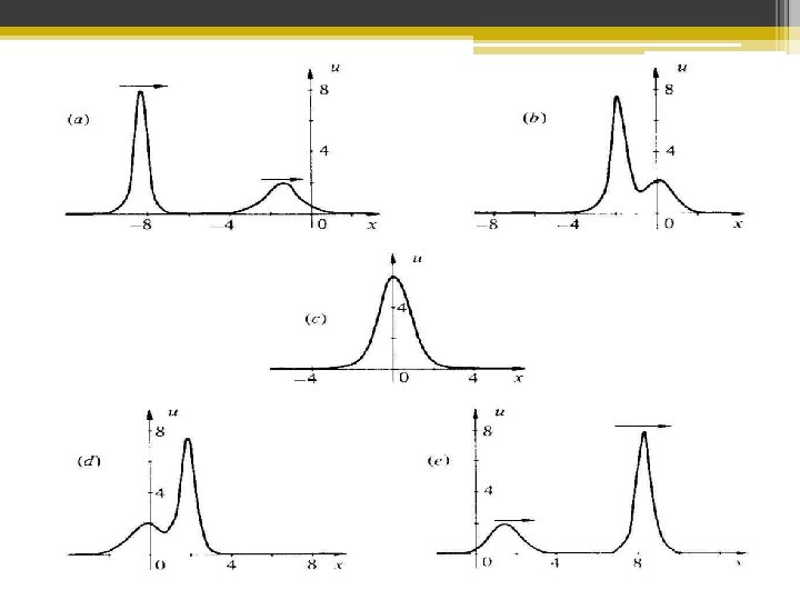
Introduction The inverse scattering transform is a method for solving some nonlinear partial differential equations. It was first introduced by Clifford S. Gardner, John M. Greene, and Martin D. Kruskal et al. (1967, 1974) for the Korteweg–de Vries equation, and soon extended to the nonlinear Schrödinger equation, the Sine-Gordon equation, and the Toda lattice equation. The method is a non-linear analogue and in some sense generalization of the Fourier transform. The name “Inverse Scattering Method” comes from the idea of recovering the time evolution of a potential from the time evolution of its scattering data.

Consider an IVP for a linear PDE (the linearized Kd. V equation) ut + uxxx = 0 , u(x , 0) = u 0(x ). (1) Assume that u(x , t ) can be expressed as a Fourier integral, u(x , t ) = Z−∞ a(k , t )eikx dk. (2) Then for (1) one finds that at = ik 3 a hence a(k , t ) = a(k , 0)eik 3 t where a(k , 0) is found as the Fourier transform of the initial condition u(x , 0). Thus the solution of the IVP (1) becomes

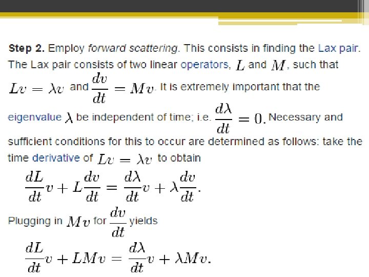
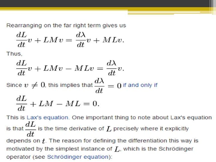
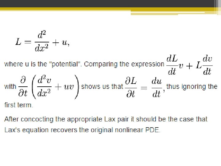
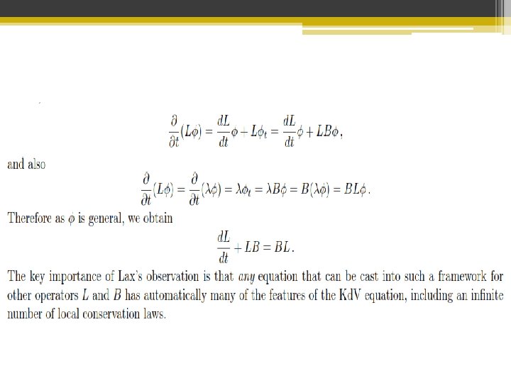
IST Method Consider an IVP for a nonlinear evolution equation ut = F (u, uxx , . . . ) , u(x , 0) = u 0(x ). (20) Assume that (20) can be represented as a compatibility condition for two linear equations Lφ φt = = λφ , Aφ. (21) (22) Let {S(λ, t )} be spectral (scattering) data for u(x , t ) in (21): the discrete eigenvalues, the norming coefficients of eigen functions, and the reflection and transmission coefficients.

Find scattering data S for the Kd. V initial condition u(x , 0) = u 0(x ) by solving φxx + (λ − u 0(x ))φ = 0. As a result we get S(0) = {κn, cn(0); a(k ; 0), b(k ; 0)}

Solving Method Step 1. Determine the nonlinear partial differential equation. This is usually accomplished by analyzing the physics of the situation being studied.

Step 3. Determine the time evolution of the eigen functions associated to each eigenvalue lambda, the norming constants, and the reflection coefficient, all three comprising the so-called scattering data. This time evolution is given by a system of linear ordinary differential equations which can be solved.

Step 4. Perform the inverse scattering procedure by solving the Gelfand–Levitan–Marchenko integral equation (Israel Moiseevich Gelfand Boris Moiseevich Levitan; [1] Vladimir Aleksandrovich Marchenko[2]), a linear integral equation, to obtain the final solution of the original nonlinear PDE. All the scattering data is required in order to do this. Note that if the reflection coefficient is zero, the process becomes much easier. Note also that this step works if L is a differential or difference operator of order two, but not necessarily for higher orders.

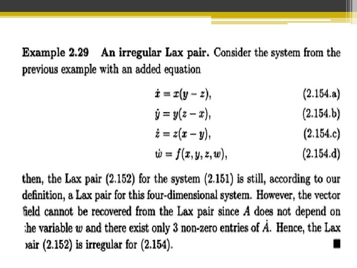
Lax-Pair Formalism

Integrable equations as compatibility conditions

From The previous equations

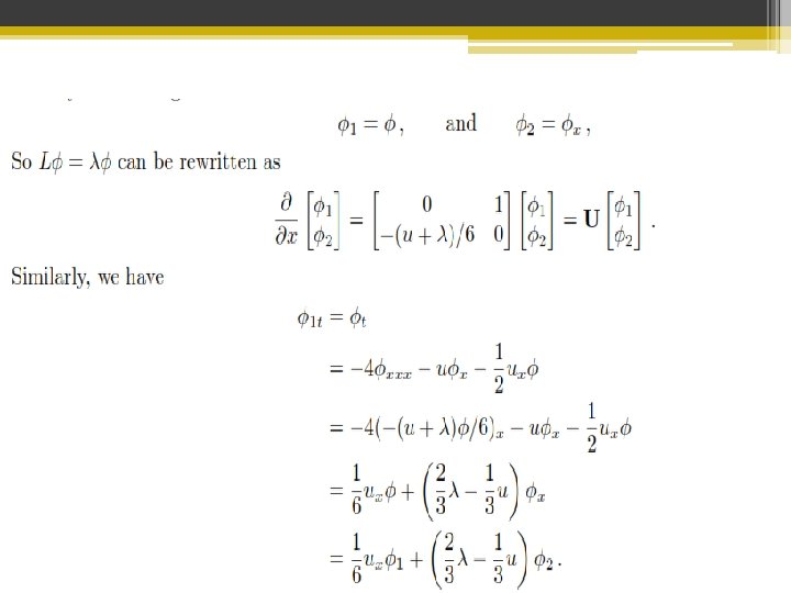
Rewriting Kd. V as a zero-curvature condition • Going further with the point of view of looking at integrable nonlinear problems as the compatibility conditions of two linear problems (frequently involving an arbitrary “spectral” parameter λ), we can go from linear operators to matrices at the cost of introducing some powers of λ. To do this, note that as the eigenvalue equation is second order, we may easily write it in first-order form by introducing:

Example

Bi-Hamiltonian Theory

Bi-Hamiltonian Systems: There are three basic (and closely related) approaches to constructing the integrals of motion required for complete integrability: • 1 - through separation of variables; • 2 - through the Lax representation; • 3 - through the bi-Hamiltonian representation.

• This system was derived from Arnol’d-Liouville theory. • While the Arnol’d-Liouville theory provides no indication on how to obtain first integrals, Hamiltonian systems admit a complete sequence of first integrals. • For a given bi-Hamiltonian system, a result owing to Magri's Theorum shows how to construct a whole hierarchy of first integrals.

Hamiltonian Mechanics Hamiltonian mechanics, a classical physical system is described by a set of canonical coordinates. r = (q, p) Canonical coordinates are a set of coordinates which can be used to describe a physical system at any given point in time.

Basic Physical Interpretation of Hamiltonian Mechanics Time evolution of the system is defined by the Hamilton’s equations: Where H = H (q, p, t) which corresponds to the total energy of the system. For a closed system, it is the sum of kinetic and potential energy.

A simple interpretation of the Hamilton’s mechanics comes from its application on one-dimensional system consisting of one particle of mass m under no external forces applied. q is the coordinate (position) and p is the momentum of the particle. T is a function of p alone and V is a function of q alone.

Magri's Theorum: • The definition of the Bi-Hamilton Systems lies in the Magri's Theorum. • "1 - The operators D & E are said to form a Hamiltonian pair if all three operators D, E & D+E are Hamiltonian. • 2 - A system of Differential equations is said to be bi. Hamiltonian with respect to the Hamiltonian pair D, E if there exist Hamiltonian functional(s) H 0 and H 1 such that the system can be written in two Hamiltonian forms: (where u = the dependent variable; H 0 and H 1 are the Hamiltonian functionals; D and E is te Hamiltonian pair. ) "

• There also exists a recursion operator R such that: • What theorem essentially suggests is as follows: Assuming is a bi. Hamiltonian system of evolution equations. Assuming that operator D is nondegenerate. Let R = E. D-1 be the corresponding recursion operator.

If we can define the differential function Then • There exists a sequence of functionals H 0, H 1, H 2, . . Such that each of the corresponding evolution equations is also a bi. Hamiltonian system.

• The Functionals Hn are in involution w. r. t either Poisson bracket: and hence provide an infinite hierarchy of conservation laws for each of the Bi-Hamiltonian systems. • The flows of bi. Hamiltonian systems all mutually commute.

Example: • Writing the following equation in Hamiltonian form:

The first form is as follows: Where Dx = D and Second form: Where And

Referances • • • Wikipedia http: //en. wikipedia. org/wiki/List_of_nonlinear_par http: //en. wikipedia. org/wiki/Inverse_scattering_transform Google Cloud converter http: //www. facebook. com/l. php? u=http%3 A%2 F%2 Fepubs. siam. or g%2 Fdoi%2 Fbook%2 F 10. 1137%2 F 1. 9781611970883&h=0 AQE 87 Qk 7 • www. math. uwaterloo. ca/~karigian/papers/ist. pdf • math. univ-lille 1. fr/~cempi/activites. . . /FR/. . . /El_IST_Lille 2014. pdf • www 2. math. ou. edu/~cremling/research/preprints/Gru. Rem. Ryb 201 4. pdftial_differential_equations

Thanks!!