Analytic Comparisons Trend Analyses Analytic Comparisons Simple comparisons

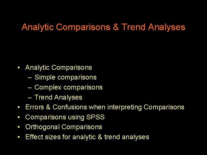
Analytic Comparisons & Trend Analyses • Analytic Comparisons – Simple comparisons – Complex comparisons – Trend Analyses • Errors & Confusions when interpreting Comparisons • Comparisons using SPSS • Orthogonal Comparisons • Effect sizes for analytic & trend analyses

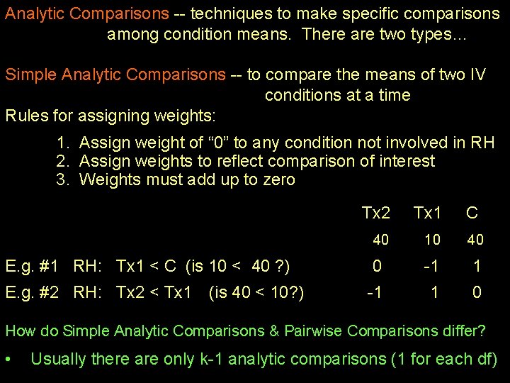
Analytic Comparisons -- techniques to make specific comparisons among condition means. There are two types… Simple Analytic Comparisons -- to compare the means of two IV conditions at a time Rules for assigning weights: 1. Assign weight of “ 0” to any condition not involved in RH 2. Assign weights to reflect comparison of interest 3. Weights must add up to zero Tx 2 Tx 1 C 40 10 40 E. g. #1 RH: Tx 1 < C (is 10 < 40 ? ) 0 -1 1 E. g. #2 RH: Tx 2 < Tx 1 (is 40 < 10? ) -1 1 0 How do Simple Analytic Comparisons & Pairwise Comparisons differ? • Usually there are only k-1 analytic comparisons (1 for each df)

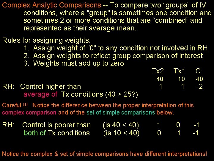
Complex Analytic Comparisons -- To compare two “groups” of IV conditions, where a “group” is sometimes one condition and sometimes 2 or more conditions that are “combined” and represented as their average mean. Rules for assigning weights: 1. Assign weight of “ 0” to any condition not involved in RH 2. Assign weights to reflect group comparison of interest 3. Weights must add up to zero Tx 2 Tx 1 C RH: Control higher than average of Tx conditions (40 > 25? ) 40 1 10 40 1 -2 Careful !!! Notice the difference between the proper interpretation of this complex comparison and of the set of simple comparisons below. RH: Control is poorer than both of Tx conditions (is 40 < 40) (is 10 < 40) 1 0 0 1 -1 -1 Notice the complex & set of simple comparisons have different interpretations!

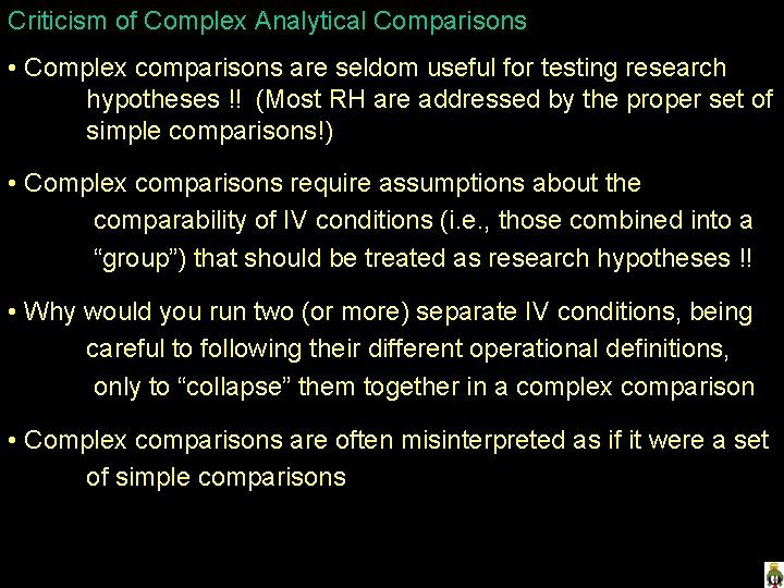
Criticism of Complex Analytical Comparisons • Complex comparisons are seldom useful for testing research hypotheses !! (Most RH are addressed by the proper set of simple comparisons!) • Complex comparisons require assumptions about the comparability of IV conditions (i. e. , those combined into a “group”) that should be treated as research hypotheses !! • Why would you run two (or more) separate IV conditions, being careful to following their different operational definitions, only to “collapse” them together in a complex comparison • Complex comparisons are often misinterpreted as if it were a set of simple comparisons

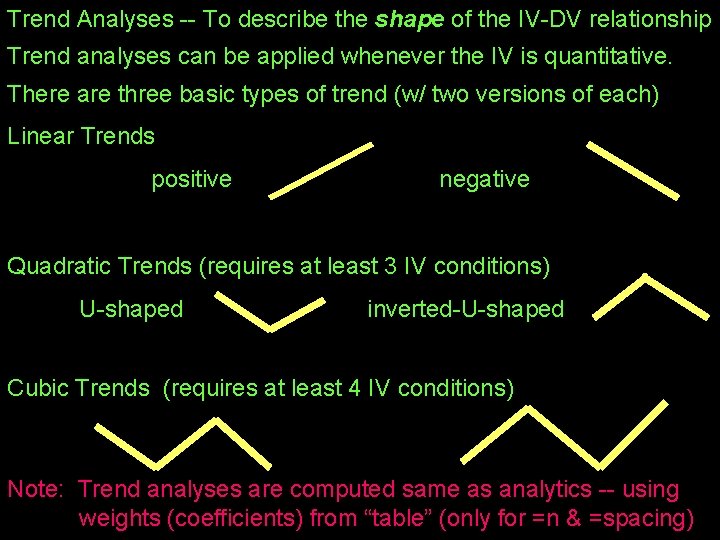
Trend Analyses -- To describe the shape of the IV-DV relationship Trend analyses can be applied whenever the IV is quantitative. There are three basic types of trend (w/ two versions of each) Linear Trends positive negative Quadratic Trends (requires at least 3 IV conditions) U-shaped inverted-U-shaped Cubic Trends (requires at least 4 IV conditions) Note: Trend analyses are computed same as analytics -- using weights (coefficients) from “table” (only for =n & =spacing)

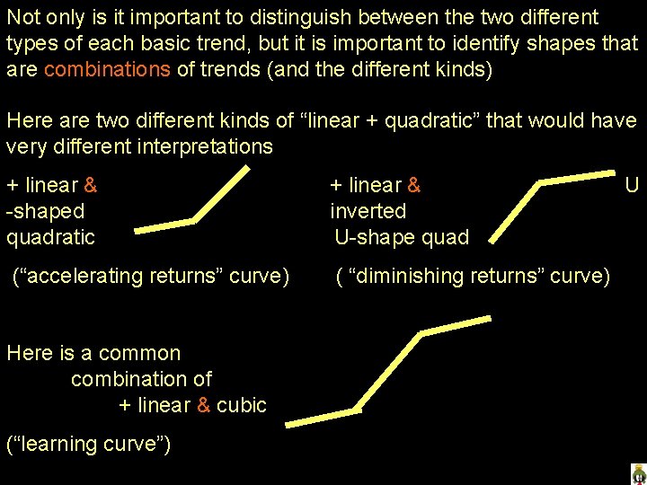
Not only is it important to distinguish between the two different types of each basic trend, but it is important to identify shapes that are combinations of trends (and the different kinds) Here are two different kinds of “linear + quadratic” that would have very different interpretations + linear & -shaped quadratic + linear & inverted U-shape quad (“accelerating returns” curve) ( “diminishing returns” curve) Here is a common combination of + linear & cubic (“learning curve”) U

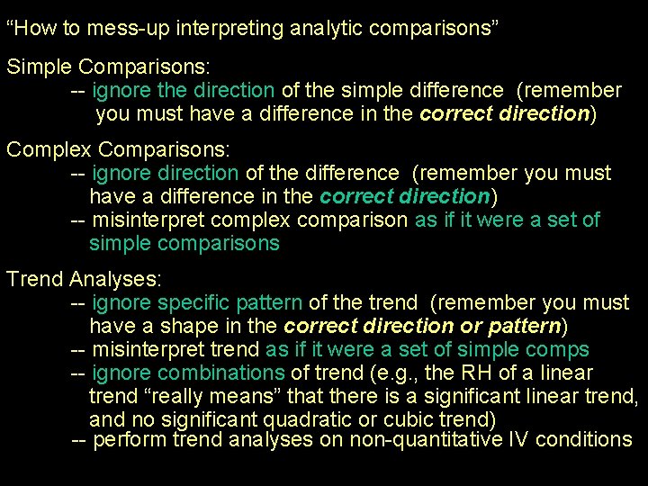
“How to mess-up interpreting analytic comparisons” Simple Comparisons: -- ignore the direction of the simple difference (remember you must have a difference in the correct direction) Complex Comparisons: -- ignore direction of the difference (remember you must have a difference in the correct direction) -- misinterpret complex comparison as if it were a set of simple comparisons Trend Analyses: -- ignore specific pattern of the trend (remember you must have a shape in the correct direction or pattern) -- misinterpret trend as if it were a set of simple comps -- ignore combinations of trend (e. g. , the RH of a linear trend “really means” that there is a significant linear trend, and no significant quadratic or cubic trend) -- perform trend analyses on non-quantitative IV conditions

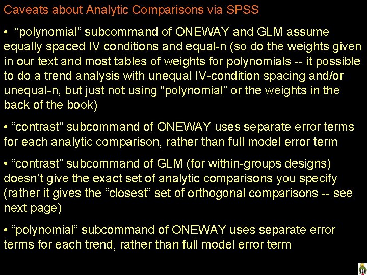
Caveats about Analytic Comparisons via SPSS • “polynomial” subcommand of ONEWAY and GLM assume equally spaced IV conditions and equal-n (so do the weights given in our text and most tables of weights for polynomials -- it possible to do a trend analysis with unequal IV-condition spacing and/or unequal-n, but just not using “polynomial” or the weights in the back of the book) • “contrast” subcommand of ONEWAY uses separate error terms for each analytic comparison, rather than full model error term • “contrast” subcommand of GLM (for within-groups designs) doesn’t give the exact set of analytic comparisons you specify (rather it gives the “closest” set of orthogonal comparisons -- see next page) • “polynomial” subcommand of ONEWAY uses separate error terms for each trend, rather than full model error term

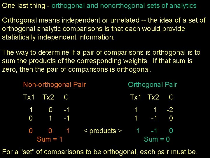
One last thing - orthogonal and nonorthogonal sets of analytics Orthogonal means independent or unrelated -- the idea of a set of orthogonal analytic comparisons is that each would provide statistically independent information. The way to determine if a pair of comparisons is orthogonal is to sum the products of the corresponding weights. If that sum is zero, then the pair of comparisons is orthogonal. Non-orthogonal Pair Orthogonal Pair Tx 1 Tx 2 C Tx 1 Tx 2 1 0 0 1 -1 -1 0 0 1 Sum = 1 1 1 < products > 1 1 -1 C -2 0 -1 0 Sum = 0 For a “set” of comparisons to be orthogonal, each pair must be.

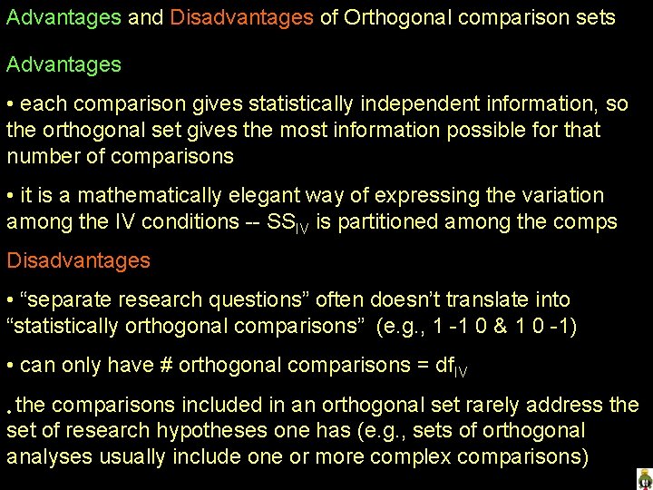
Advantages and Disadvantages of Orthogonal comparison sets Advantages • each comparison gives statistically independent information, so the orthogonal set gives the most information possible for that number of comparisons • it is a mathematically elegant way of expressing the variation among the IV conditions -- SSIV is partitioned among the comps Disadvantages • “separate research questions” often doesn’t translate into “statistically orthogonal comparisons” (e. g. , 1 -1 0 & 1 0 -1) • can only have # orthogonal comparisons = df. IV • the comparisons included in an orthogonal set rarely address the set of research hypotheses one has (e. g. , sets of orthogonal analyses usually include one or more complex comparisons)

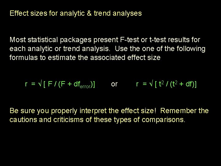
Effect sizes for analytic & trend analyses Most statistical packages present F-test or t-test results for each analytic or trend analysis. Use the one of the following formulas to estimate the associated effect size r = [ F / (F + dferror)] or r = [ t 2 / (t 2 + df)] Be sure you properly interpret the effect size! Remember the cautions and criticisms of these types of comparisons.