Analytic Analysis of Differential Equations Generally realworld differential

Analytic Analysis of Differential Equations

Generally real-world differential equations are not directly solvable. That's when we use numerical approximations. We're going to look at some simple ones to get a better understanding of the differential equations themselves.

Differential Equations contain the derivatives of unknown functions. Given some simple differential equations, we can sometimes guess at the form of the function. So we will work backwards – from the solution to the differential equation.

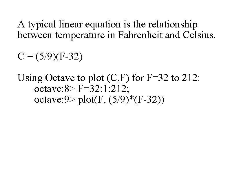
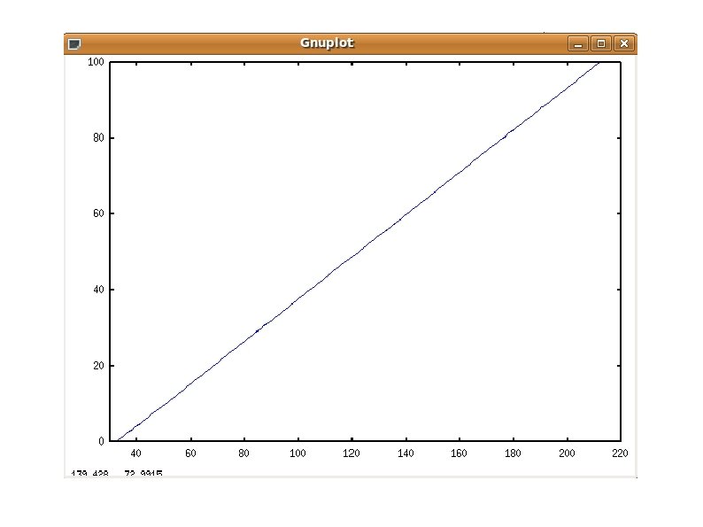
A typical linear equation is the relationship between temperature in Fahrenheit and Celsius. C = (5/9)(F-32) Using Octave to plot (C, F) for F=32 to 212: octave: 8> F=32: 1: 212; octave: 9> plot(F, (5/9)*(F-32))

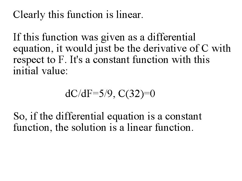
Clearly this function is linear. If this function was given as a differential equation, it would just be the derivative of C with respect to F. It's a constant function with this initial value: d. C/d. F=5/9, C(32)=0 So, if the differential equation is a constant function, the solution is a linear function.

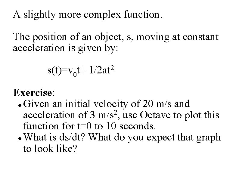
A slightly more complex function. The position of an object, s, moving at constant acceleration is given by: s(t)=v 0 t+ 1/2 at 2 Exercise: Given an initial velocity of 20 m/s and acceleration of 3 m/s 2, use Octave to plot this function for t=0 to 10 seconds. What is ds/dt? What do you expect that graph to look like?

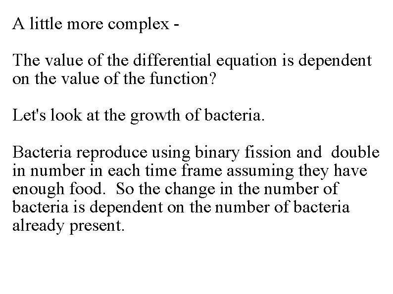
A little more complex The value of the differential equation is dependent on the value of the function? Let's look at the growth of bacteria. Bacteria reproduce using binary fission and double in number in each time frame assuming they have enough food. So the change in the number of bacteria is dependent on the number of bacteria already present.

Exercise: Assume our example bacteria doubles every ten minutes and has plenty to consume. Starting with one bacteria, use Octave to plot the number of bacteria every ten minutes for two hours. How many bacteria are there after two hours?

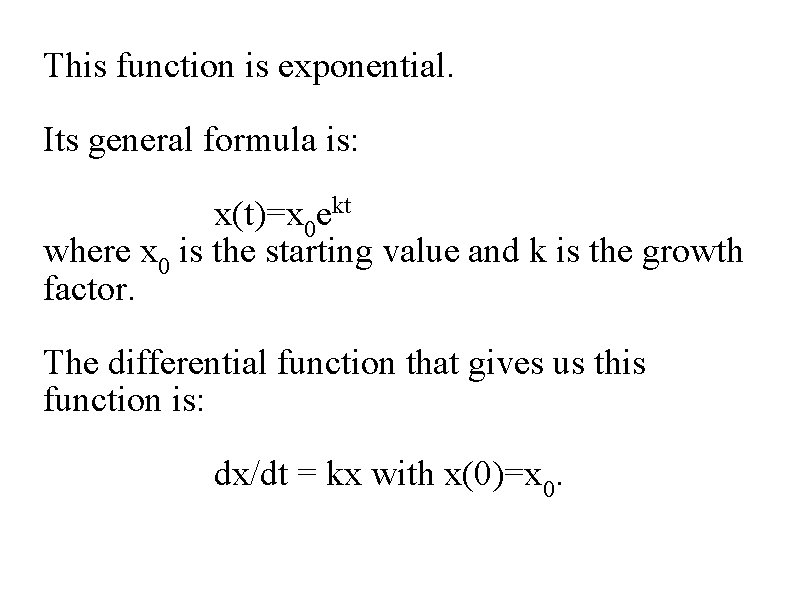
This function is exponential. Its general formula is: x(t)=x 0 ekt where x 0 is the starting value and k is the growth factor. The differential function that gives us this function is: dx/dt = kx with x(0)=x 0.

So testing this out - another population example: Population is not often based solely on population growth, but also on predation. Assume there is an population of animals, x. They have a growth rate, r, that depends on their birth rate.

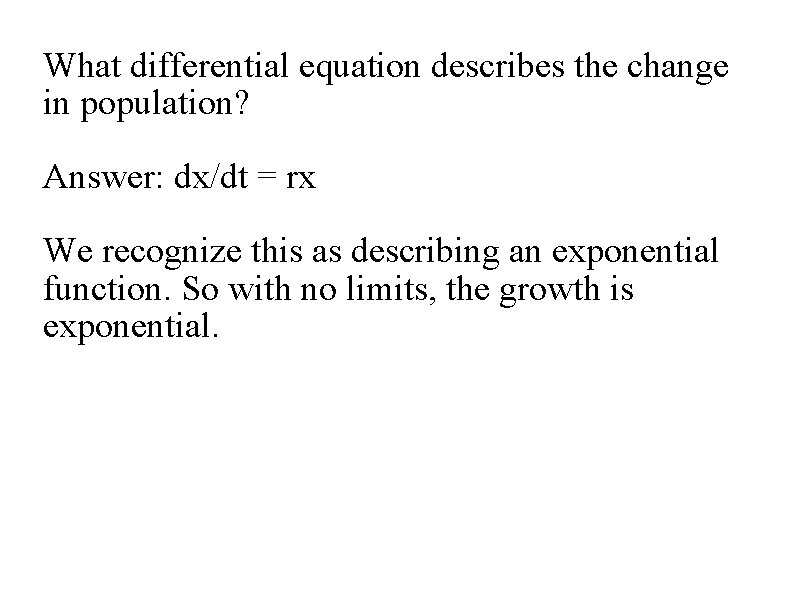
What differential equation describes the change in population? Answer: dx/dt = rx We recognize this as describing an exponential function. So with no limits, the growth is exponential.

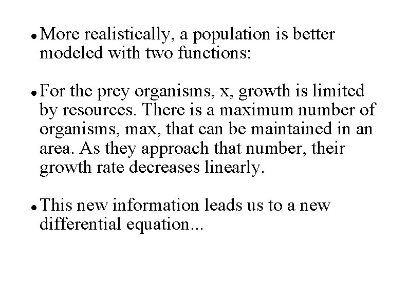
More realistically, a population is better modeled with two functions: For the prey organisms, x, growth is limited by resources. There is a maximum number of organisms, max, that can be maintained in an area. As they approach that number, their growth rate decreases linearly. This new information leads us to a new differential equation. . .

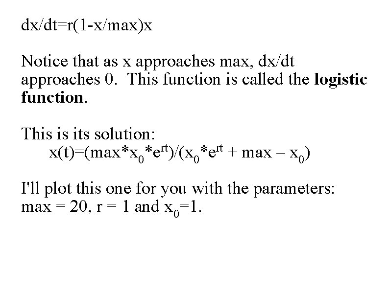
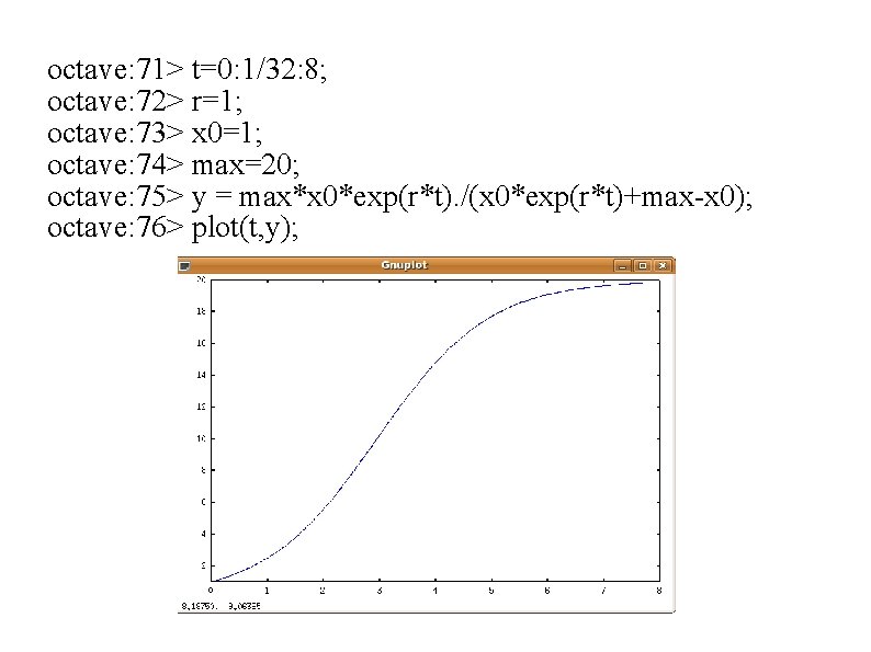
dx/dt=r(1 -x/max)x Notice that as x approaches max, dx/dt approaches 0. This function is called the logistic function. This is its solution: x(t)=(max*x 0*ert)/(x 0*ert + max – x 0) I'll plot this one for you with the parameters: max = 20, r = 1 and x 0=1.

octave: 71> t=0: 1/32: 8; octave: 72> r=1; octave: 73> x 0=1; octave: 74> max=20; octave: 75> y = max*x 0*exp(r*t). /(x 0*exp(r*t)+max-x 0); octave: 76> plot(t, y);

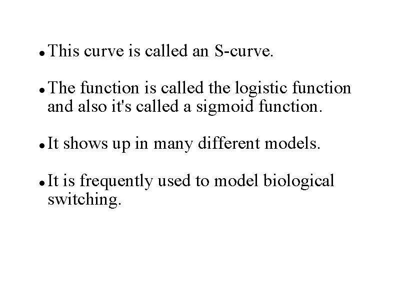
This curve is called an S-curve. The function is called the logistic function and also it's called a sigmoid function. It shows up in many different models. It is frequently used to model biological switching.

But organisms do not tend to live alone. If they are prey, they live with predators. Now the growth of the prey, x, is affected by the number of predators, y. And the growth of the predators is affected by the number of prey. Now we have a system of differential equations that depend on each other.

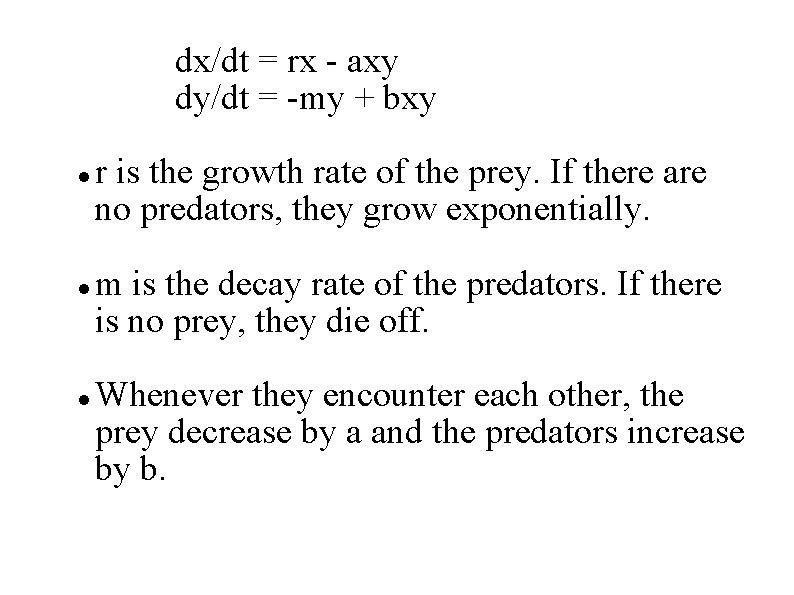
dx/dt = rx - axy dy/dt = -my + bxy r is the growth rate of the prey. If there are no predators, they grow exponentially. m is the decay rate of the predators. If there is no prey, they die off. Whenever they encounter each other, the prey decrease by a and the predators increase by b.

We cannot write a formula to express the solution to this system of equations. We could use numerical methods to approximate a solution, but we can't find one analytically.

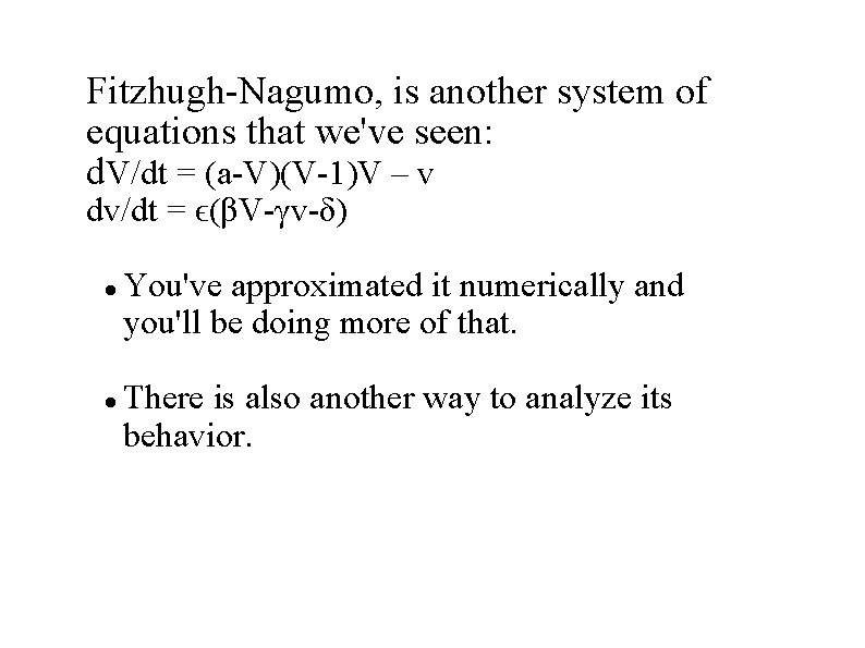
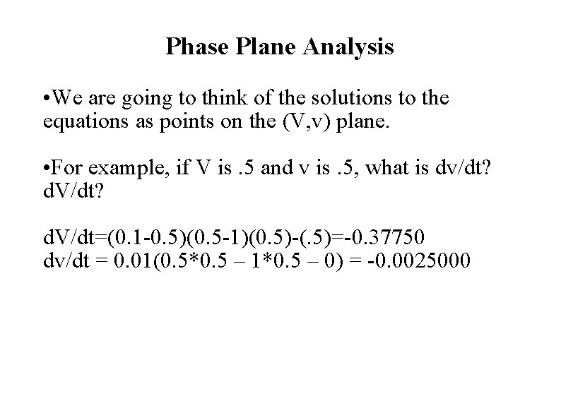
Fitzhugh-Nagumo, is another system of equations that we've seen: d. V/dt = (a-V)(V-1)V – v dv/dt = ϵ(βV-γv-δ) You've approximated it numerically and you'll be doing more of that. There is also another way to analyze its behavior.

Phase Plane Analysis • We are going to think of the solutions to the equations as points on the (V, v) plane. • For example, if V is. 5 and v is. 5, what is dv/dt? d. V/dt=(0. 1 -0. 5)(0. 5 -1)(0. 5)-(. 5)=-0. 37750 dv/dt = 0. 01(0. 5*0. 5 – 1*0. 5 – 0) = -0. 0025000

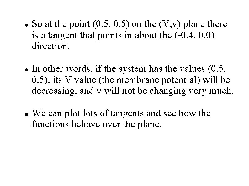
So at the point (0. 5, 0. 5) on the (V, v) plane there is a tangent that points in about the (-0. 4, 0. 0) direction. In other words, if the system has the values (0. 5, 0, 5), its V value (the membrane potential) will be decreasing, and v will not be changing very much. We can plot lots of tangents and see how the functions behave over the plane.

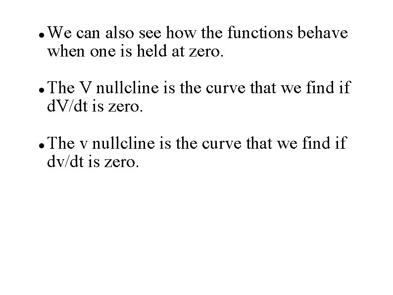
We can also see how the functions behave when one is held at zero. The V nullcline is the curve that we find if d. V/dt is zero. The v nullcline is the curve that we find if dv/dt is zero.

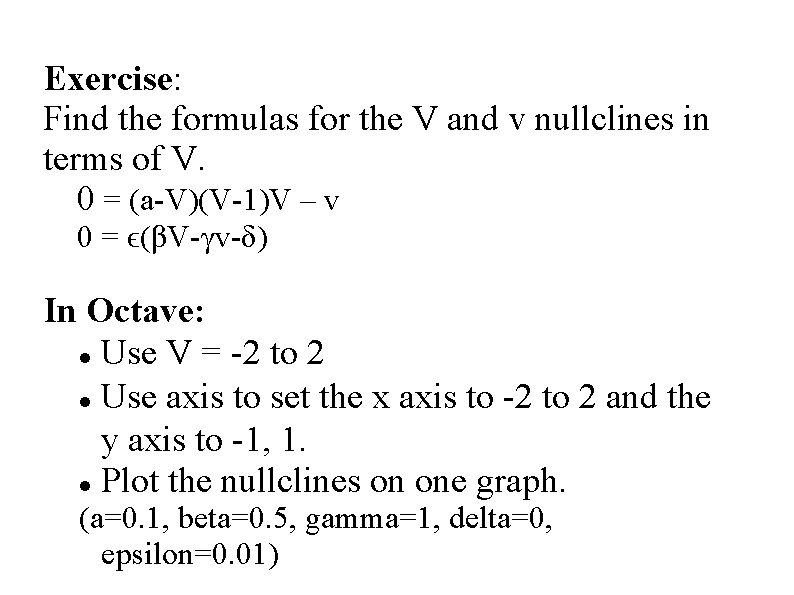
Exercise: Find the formulas for the V and v nullclines in terms of V. 0 = (a-V)(V-1)V – v 0 = ϵ(βV-γv-δ) In Octave: Use V = -2 to 2 Use axis to set the x axis to -2 to 2 and the y axis to -1, 1. Plot the nullclines on one graph. (a=0. 1, beta=0. 5, gamma=1, delta=0, epsilon=0. 01)

We can look at a simulation of the Fitzhugh. Nagumo phase plane at thevirtualheart. org. The applet on top shows the phase plane along with the tangent lines. Click on a starting point to see how the system behaves. The applet on the bottom plots V (U) and v over time. http: //thevirtualheart. org/java/fhnphase. html

Exercises: Try the parameter changes suggested on the page. Try to determine, the minimum value of delta that will make the system autooscillatory. How does the intersection point of the two nullclines relate to the behavior of the system?