Analysis of Variance in Matrix form The ANOVA

Analysis of Variance in Matrix form • The ANOVA table sums of squares, SSTO, SSR and SSE can all be expressed in matrix form as follows…. week 9 1

Multiple Regression • A multiple regression model is a model that has more than one explanatory variable in it. • Some of the reasons to use multiple regression models are: Ø Often multiple X’s arise naturally from a study. Ø We want to control for some X’s Ø Want to fit a polynomial Ø Compare regression lines for two groups week 9 2

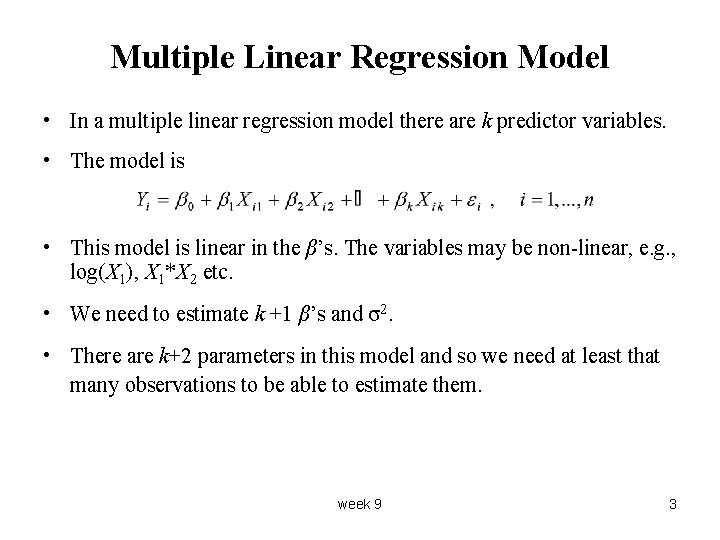
Multiple Linear Regression Model • In a multiple linear regression model there are k predictor variables. • The model is • This model is linear in the β’s. The variables may be non-linear, e. g. , log(X 1), X 1*X 2 etc. • We need to estimate k +1 β’s and σ2. • There are k+2 parameters in this model and so we need at least that many observations to be able to estimate them. week 9 3

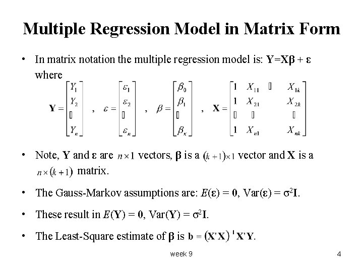
Multiple Regression Model in Matrix Form • In matrix notation the multiple regression model is: Y=Xβ + ε where • Note, Y and ε are matrix. vectors, β is a vector and X is a • The Gauss-Markov assumptions are: E(ε) = 0, Var(ε) = σ2 I. • These result in E(Y) = 0, Var(Y) = σ2 I. • The Least-Square estimate of β is week 9 4

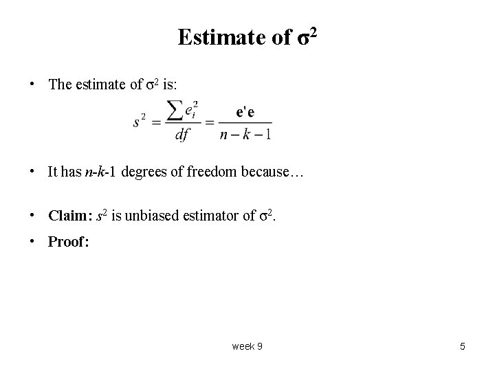
Estimate of σ2 • The estimate of σ2 is: • It has n-k-1 degrees of freedom because… • Claim: s 2 is unbiased estimator of σ2. • Proof: week 9 5

General Comments about Multiple Regression • The regression equation gives the mean response for each combination of explanatory variables. • The regression equation will not be useful if it is very complicated or a function of large number of explanatory variables. • We generally want “parsimonious” model, that is, a model that is as simple as possible to adequately describe the response variable. • It is unwise to think that there is some exact, discoverable equation. • Many possible models are available. • One or two models may adequately approximate the mean of the response variable. week 9 6

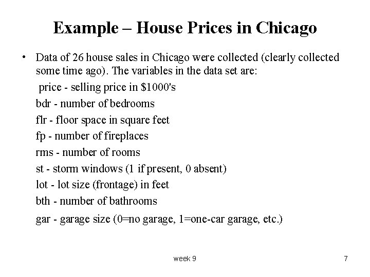
Example – House Prices in Chicago • Data of 26 house sales in Chicago were collected (clearly collected some time ago). The variables in the data set are: price - selling price in $1000's bdr - number of bedrooms flr - floor space in square feet fp - number of fireplaces rms - number of rooms st - storm windows (1 if present, 0 absent) lot - lot size (frontage) in feet bth - number of bathrooms gar - garage size (0=no garage, 1=one-car garage, etc. ) week 9 7

Interpreting Regression Coefficients • b 0 is the estimate of the mean value of Y when all the predictor variables are 0; it may be meaningless in many cases. • bj , j = 1, …, k is the estimated change in Y, on average, due to a unit increase in Xj where all the other variables held fixed. Note, that it may be impossible to hold all other variables fixed. • Example, re the home price example above, for 100 extra square feet (everything else held constant), the price goes up by $1760 on average. For one more room (everything else held constant), the price goes up by $3900 on average. For one more bedroom (everything else held constant), the price goes down by $7700 on average. week 9 8

Residual Plots • As in the simple linear regression model, we examine 3 types of residual plots to assess the validity of the model assumptions. • The plots are: Ø Residual versus Xj , j = 1, …, k. We examine presence of curvature and/or influential points. Ø Residual versus predicted values. We use this plot to check for non-constant variance and for any outliers in residuals. Ø Normal quantile plot of residuals. week 9 9

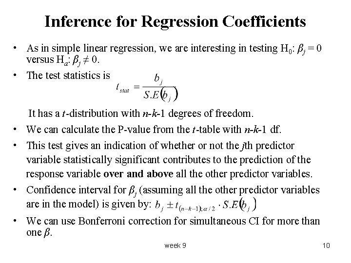
Inference for Regression Coefficients • As in simple linear regression, we are interesting in testing H 0: βj = 0 versus Ha: βj ≠ 0. • The test statistics is It has a t-distribution with n-k-1 degrees of freedom. • We can calculate the P-value from the t-table with n-k-1 df. • This test gives an indication of whether or not the jth predictor variable statistically significant contributes to the prediction of the response variable over and above all the other predictor variables. • Confidence interval for βj (assuming all the other predictor variables are in the model) is given by: • We can use Bonferroni correction for simultaneous CI for more than one β. week 9 10

ANOVA Table • The ANOVA table in multiple regression model is given by… week 9 11

Coefficient of Multiple Determination – R 2 • As in simple linear regression model, R 2 = SSR/SSTO. • In multiple regression this is called the “coefficient of multiple determination”; it is not the square of a correlation coefficient. • In multiple regression, R 2 always goes up when more predictor variables are added to the model, regardless of whether the predictor variables are useful in estimating Y. week 9 12

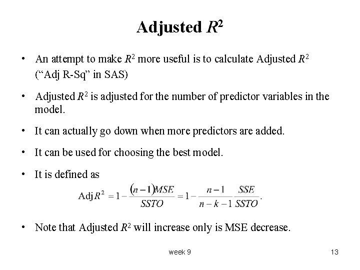
Adjusted R 2 • An attempt to make R 2 more useful is to calculate Adjusted R 2 (“Adj R-Sq” in SAS) • Adjusted R 2 is adjusted for the number of predictor variables in the model. • It can actually go down when more predictors are added. • It can be used for choosing the best model. • It is defined as • Note that Adjusted R 2 will increase only is MSE decrease. week 9 13