Analysis of Variance CSLU 2850 Lo 1 Spring

Analysis of Variance CSLU 2850. Lo 1 Spring 2008 Cameron Mc. Inally mcinally@fordham. edu Fordham University May contain work from the Creative Commons.

Analysis of Variance • Analysis of Variance § § In the Statistical Inference section, we studied how a two-sample t-test can be used to determine whether a significant difference exists between the samples. Now, we will use Analysis of Variance to compare the means of two or more samples.

Analysis of Variance • Null and Alternative Hypotheses § § § H 0 : μ 1 = μ 2 = … = μ n HA: Not all of the μi are equal. Here, there are n samples and μi is the mean of the ith sample.

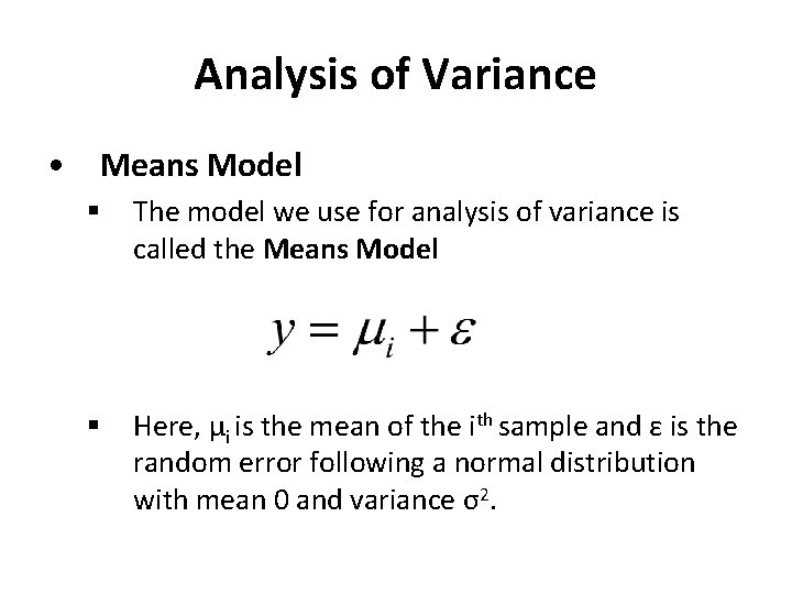
Analysis of Variance • Means Model § The model we use for analysis of variance is called the Means Model § Here, μi is the mean of the ith sample and ε is the random error following a normal distribution with mean 0 and variance σ2.

Analysis of Variance • Necessary Assumptions § § § The errors are normally distributed. The errors are independent. The errors have constant variance, σ2.

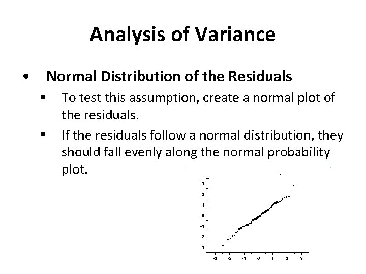
Analysis of Variance • Normal Distribution of the Residuals § § To test this assumption, create a normal plot of the residuals. If the residuals follow a normal distribution, they should fall evenly along the normal probability plot.

Analysis of Variance • Independent errors § § This final assumption should only be considered when there is a defined order of the observations. We would like to make sure that the residual of a data point is not influenced by the surrounding data points.

Analysis of Variance • Constant variance assumption § § § Next, we will look at the assumption of constant variance in the residuals. To view this graphically, plot the residual values against the predicted values. If there is an increase in variance, at any point along the line, then there is reason to doubt the assumption of constant variance. Outliers may have a significant impact on this test.

Analysis of Variance • Ao. V and Regression § § § Analysis of Variance is a special form of Regression. In the case of Analysis of Variance, the predictor variables are discrete, rather than continuous. To express an Analysis of Variance in terms of Regression, we must reformulate the model.

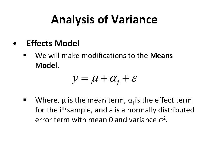
Analysis of Variance • Effects Model § We will make modifications to the Means Model. § Where, μ is the mean term, αi is the effect term for the ith sample, and ε is a normally distributed error term with mean 0 and variance σ2.

Analysis of Variance • Two-way Analysis of Variance § § One-way Analysis of Variance compares several samples corresponding to a factor. Two-way Analysis of Variance uses two factors, e. g. medication and dose in a medical experiment.

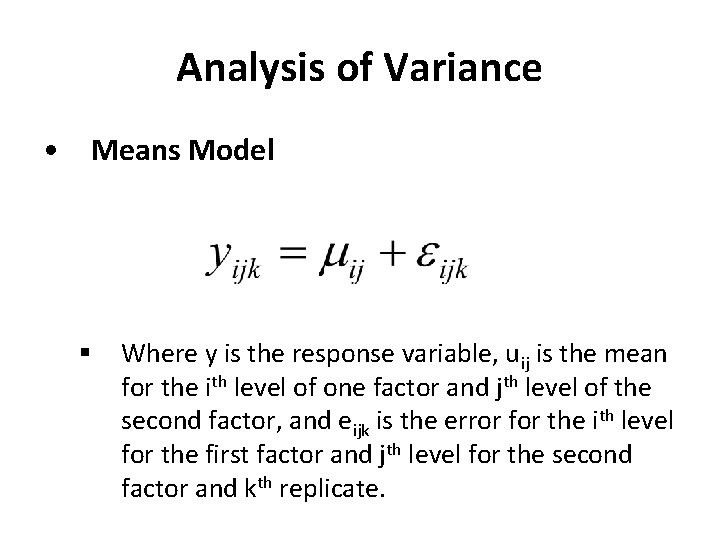
Analysis of Variance • Means Model § Where y is the response variable, uij is the mean for the ith level of one factor and jth level of the second factor, and eijk is the error for the ith level for the first factor and jth level for the second factor and kth replicate.

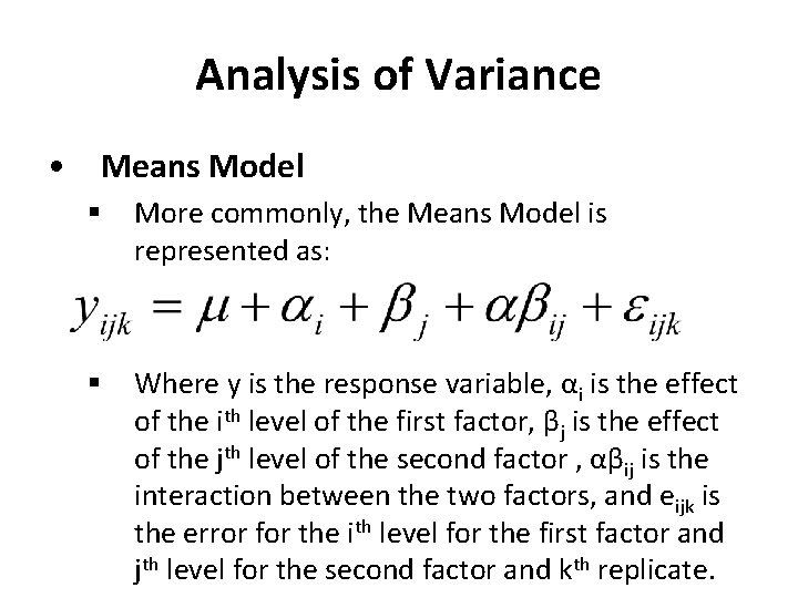
Analysis of Variance • Means Model § More commonly, the Means Model is represented as: § Where y is the response variable, αi is the effect of the ith level of the first factor, βj is the effect of the jth level of the second factor , αβij is the interaction between the two factors, and eijk is the error for the ith level for the first factor and jth level for the second factor and kth replicate.

Analysis of Variance Homework (Always Due in One Week) Week • Read Chapter 10. • Complete Chapter 10, pg. 400: 1 (a-d), 4